Analysis of Gearbox Losses for High-Performance Electric Motorcycle Applications ^†

Abstract

Finding an architectural solution that satisfies electric motorcycles’ performance and riding range is challenging due to the electric powertrain constraints, such as low battery energy density. This paper analyzes the gearbox and powertrain efficiency for battery electric motorcycles (BEMs) based on the drivetrain architecture and under various vehicle use scenarios. The impact on the consumption of a constant-speed gearbox is investigated, focusing mainly on load-independent losses. The analysis is performed using an analytic approach and experimental data. Two different gearbox and powertrain solutions are characterized through test bench experiments, running them under free-driving conditions and no-load tests. A comparison of these powertrain solutions in terms of consumption for the same motorcycle model under different speed profiles (WMTC, LA-4) is conducted. The results show the energy losses and provide information for defining drivetrain components and architectures.

1. Introduction

The production of Battery Electric Vehicles (BEVs) has increased in recent years for many reasons [1], including their lower CO₂ emissions compared to conventional vehicles. Consolidated architecture is not yet clear in the case of high-performance electric motorcycles. The flexibility of the electric powertrain allows for different vehicle topologies, such as two-wheel-driven vehicles. However, a BEV has other issues, like lithium batteries’ lower specific energy density than fossil fuels. The riding range can increase with the battery capacity, while vehicle consumption always increases as a result of an increase in mass caused by a larger battery size. If the electric machine works as a generator during vehicle braking (regenerative braking), a significant amount of kinetic energy could be recovered, extending the riding range [2]. Increasing overall efficiency also means a higher riding range for the same vehicle, which can be achieved by reducing the number of gear stages or using a direct hub wheel motor. The latter motor increases the unsprung mass, and motor cooling can be challenging. The electric torque generated by the motor for a permanent magnet AC machine is proportional to the product of magnetic loading, electric loading, and rotor volume [3]. The same electric machine power can be obtained with high torque and low speed or vice versa (a high-speed machine). The power density increases at high speeds [4], although the torque is reduced. A high-speed motor requires less volume and mass for a given power. A gearbox might be needed to match the motor to the vehicle’s operating range, despite a lower maximum torque that can be supplied. Electric motorcycles have limited onboard volume compared to cars or trucks, so a high-speed machine can help reduce the volume needed by the powertrain, albeit with an increase in the loss density. Losses can be avoided or reduced using better and more expensive materials and different designs, although a better heat extraction system (cooling system) might be needed. The high-speed machine coupled with a gearbox is the most commonly used solution, as used by Energica and Ducati for their respective MotoE motorcycles.

In this work, the losses caused by the gearbox are analyzed under free-load or non-driving conditions. The powertrain consists of an electric machine coupled to the gearbox with an integrated frame, so the full disengagement of the latter machine is impossible. The electric machine loss impacts vehicle consumption, and the procedure for estimating the riding range for the electric motorcycle is modified to account for this [5]. To allow the vehicle to coast down, the electric machine must work as a motor to equalize the inherent losses. These latter losses in a Surface Permanent Magnet Synchronous Machine (SPMSM) include copper loss (Joule effect), iron or core loss (hysteresis and eddy current), permanent magnet loss, friction, and windage loss [6]. Other sources of losses in this powertrain are due to inverter, gearbox loss, and stray loss (nonuniform harmonic distribution). No-load losses are measured at constant speed, and their influence on consumption on the driving cycles (UDSS, WMTC) is investigated. Battery loss is not investigated in the experimental test.

2. Materials and Methods

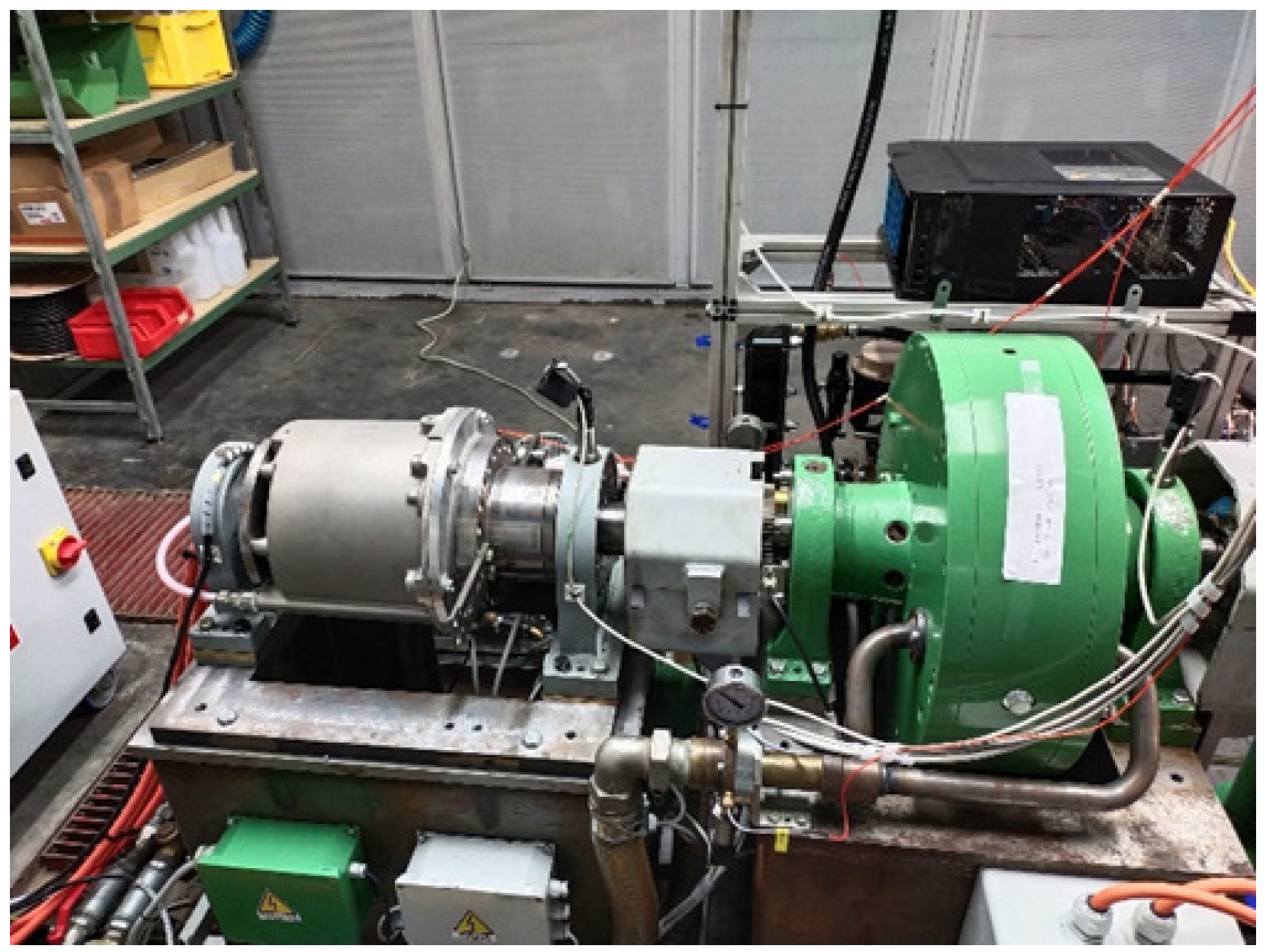
2.1. Test Bench and Setup

The powertrain characterized by the experimental test consisted of an inverter, an electric machine, and a gearbox. The layout of the system is shown in Figure 1. The heat was extracted by the cooling system, despite the low power generated by the motor during the no-load test.

The gearbox consisted of a single-speed configuration with three reduction stages. The gearbox was mated directly and rigidly with the motor shaft and then joined to the bench motor via a coupling. This latter motor acted as the resistive vehicle load during the motoring phase of the powertrain and is shown in Figure 2. The torque applied to the coupling was recorded via load cells, and the motor speed was recorded by an encoder. The power loss was calculated as the product of the torque and speed. A battery simulator device was used to power the electric drive.

2.2. No-Load Losses

The no-load test consisted of a zero resistance torque by the electric machine ($T_m=0$), so the input power provided by the bench was ideally equal to only the gearbox loss. The motor losses included stator copper loss, core loss (i.e., hysteresis and eddy currents), permanent magnet loss in the rotor, friction loss (dry friction, bearing, sealing), windage loss, and stray loss. The no-load test involved driving the motor at a constant speed with zero torque delivered. Because of the gearbox loss and imprecision in zero-torque control, an external torque delivered by the bench was needed to maintain the target speed. This latter torque was measured on the gearbox shaft. The power loss was calculated as the product of the torque measured at the gearbox output and the speed at the same measurement point. The copper loss usually accounts for the main part of the electric motor losses, especially at low speeds. In the free-driving condition, the stator current was near zero and so too was the copper loss. The gearbox has a single fixed-speed configuration with three cylindrical gear stages. The power loss in the gearbox was described in [7], where the power loss was calculated based on the thermal equilibrium between the gearbox and the dissipated heat. In general, the power loss in the gearbox consists of load-dependent and no-load-dependent losses in the gears and bearings, as well as load-independent losses in the gears and lubrication. Decoupling all these loss terms was not possible in a single test with the available equipment, as done in [8,9]. The experimental data provided the total loss of power as a function of speed, neglecting the copper loss (a function of the current, and thus of torque) and the gearbox load-dependent loss due to the low torque applied during the test.

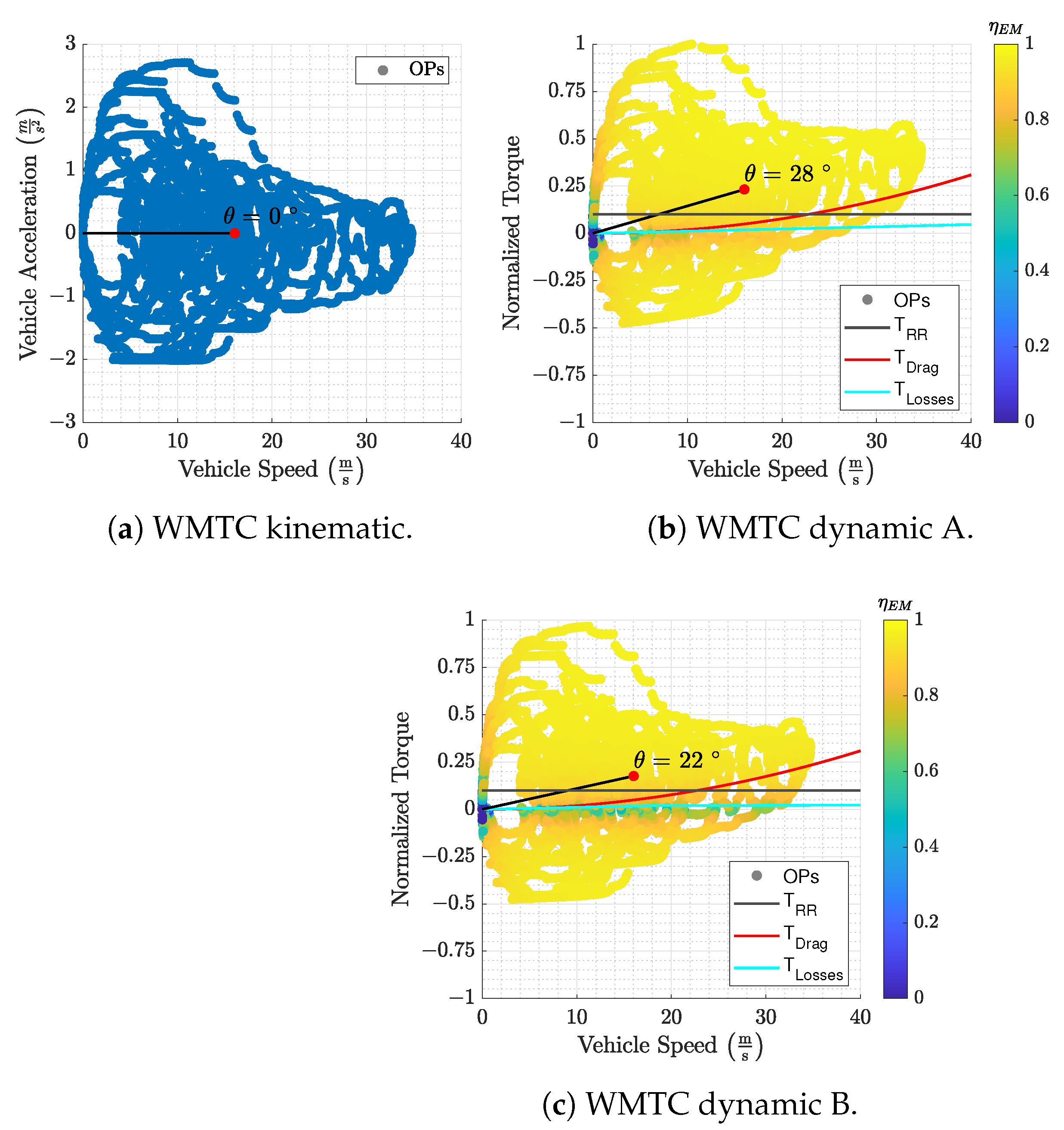
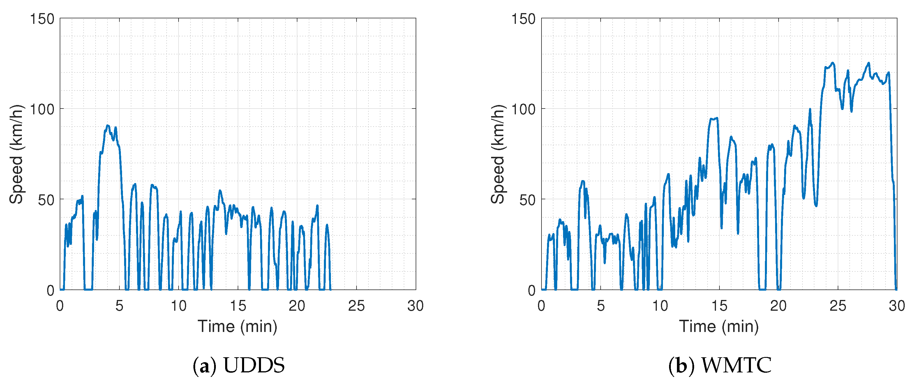
2.3. Vehicle Model and Speed Profiles

The longitudinal vehicle dynamics were modeled via a 1 DoF approximation, and the vehicle parameters, like mass, were kept constant. The traction force ($F_T$) acting on the vehicle is given by Equation (1) [10]:

$$F_T\left(t\right)={\displaystyle \frac{1}{2}}\rho A{C}_{d}v{\left(t\right)}^2+ma\left(t\right)+mg{c}_{rr}$$

(1)

where the first term on the right side is the aerodynamic resistance, the second term is the inertia resistance, and the last term is the tire rolling resistance. The mechanical energy spent by the vehicle is given by Equation (2) as the power traction integral over time. The battery energy can be calculated considering all the efficiencies of the powertrain components, including the battery itself.

$$E_T\left(t\right)={\int }_0^t{P}_T\left(\tau \right)d\tau ={\int }_0^t{F}_T\left(\tau \right)v\left(\tau \right)d\tau$$

(2)

The influence of free-driving losses on consumption was evaluated using the vehicle model to describe the vehicle dynamics and different speed profiles, which describe the vehicle’s kinematics. Consumption was calculated as the battery energy expended by the vehicle to overcome the resistance force, normalized by the distance traveled. Two speed profiles were used as input: the Urban Dynamometer Driving Schedule (UDDS), called LA-4, and the World Motorcycle Test Cycle (WMTC). These speed profiles are well known and used for estimating the consumption of both conventional and electric vehicles according to different standards. The speed profiles are shown in Figure 3. The powertrain components, such as the battery and the final drive transmission, were modeled in the Matlab/Simulink environment following experimental characterization.

3. Results

3.1. Free-Driving Losses

The resistance torques, normalized by the maximum value, for the two powertrains (A, B) are shown in Figure 4. Powertrain B exhibited a monotonic trend and was approximated with a linear piecewise function, a behavior similar to that observed in other works [11,12]. The torque resistance of powertrain A was almost equal to that of B from 0 to 15 km/h and could be considered linear up to 100 km/h with a small error. Powertrain A reached the maximum value at 116 km/h, which then decreased with increasing speed.

The normalized resistance power for the two powertrains and their difference are shown in Figure 5. The power loss of powertrain B had a quadratic relation with the speed due to the linearity relation of the torque resistance. Although the resistance torque for powertrain A decreased after 116 km/h, the resistance power increased, reaching its maximum value at 221 km/h.

As long as the torque decreased at a rate lower than linear with speed, the product of torque and speed increased (indicating a positive first derivative).

3.2. Energy Consumption

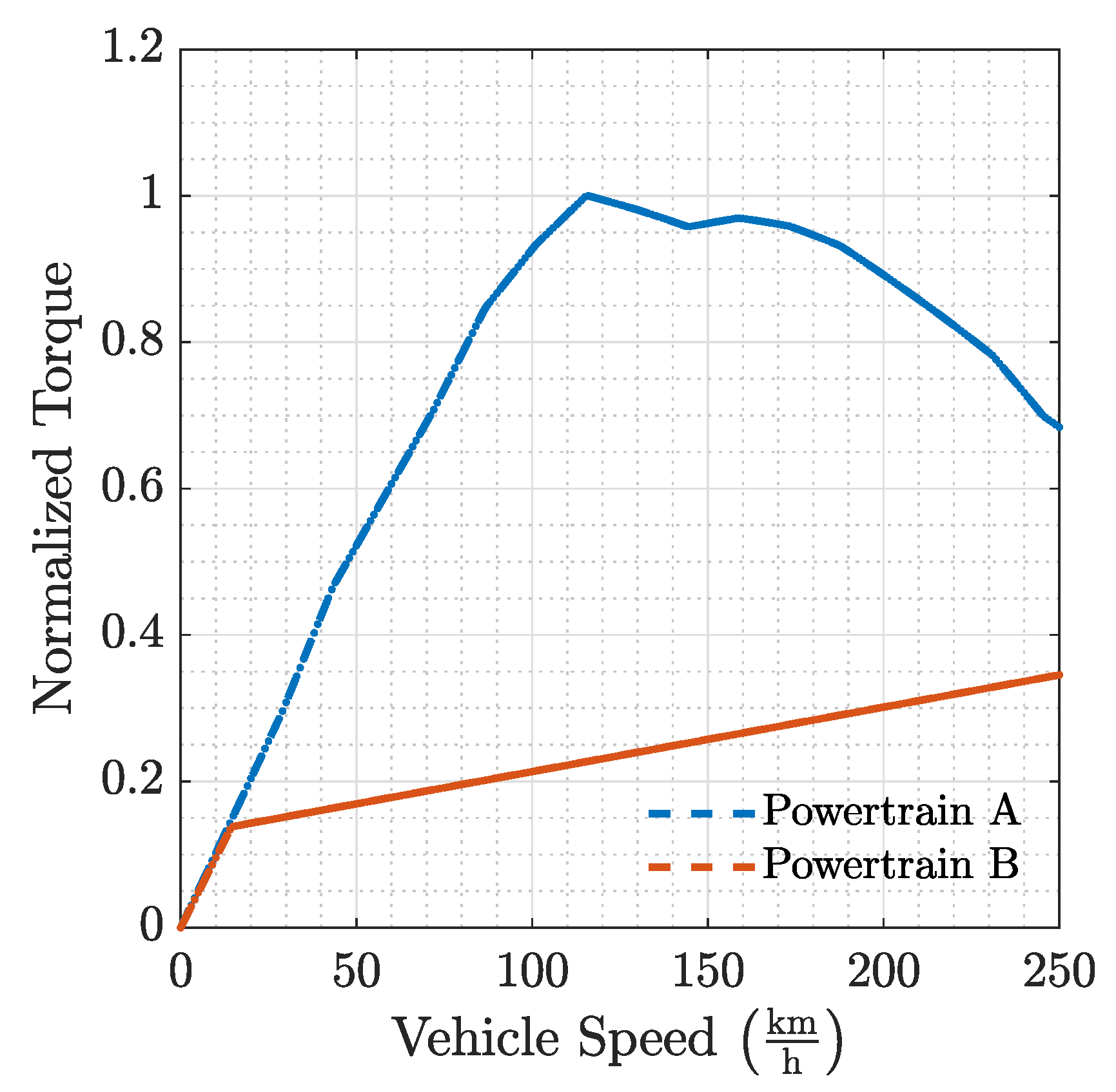
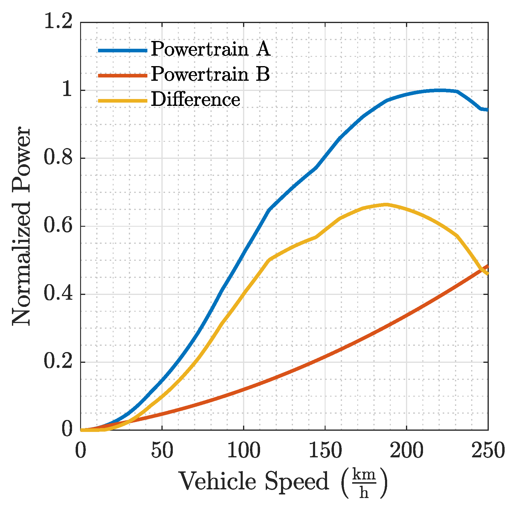
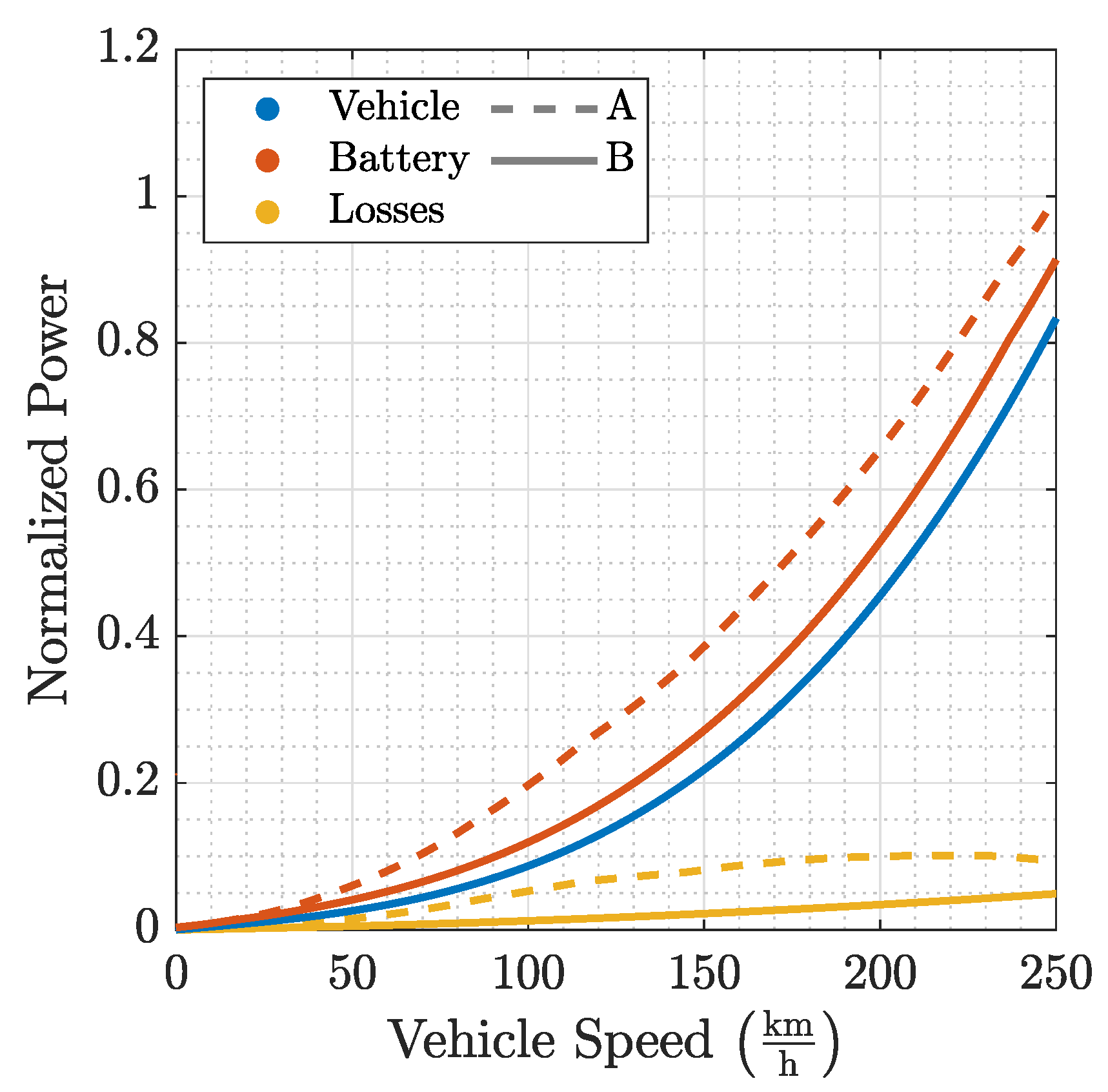
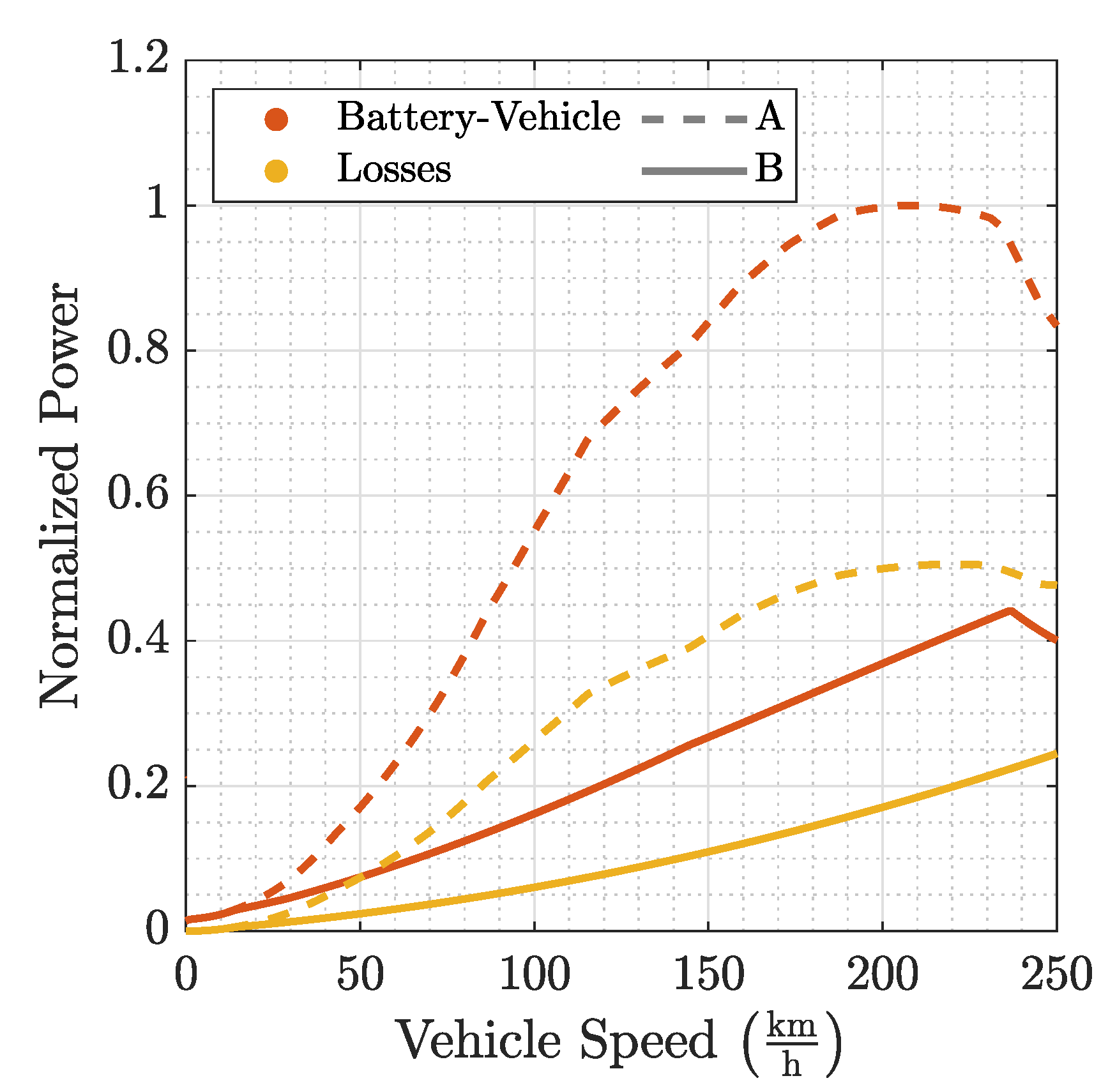
The normalized consumption was obtained through the vehicle model and the speed profiles described in Section 2.3 for powertrains A and B. The vehicle parameters were kept constant for both vehicle models and therefore the mechanical power demand was the same. The front vehicle cross-section did not change, nor did the mass, due to the small differences between the architectures, so the analysis focused only on the free-rolling difference. Figure 6 shows the power needed by the vehicle as a function of the speed. The power required by the vehicle was the same for both powertrain models, while the battery power differed due to varying losses and shifts in operating points (e.g., different efficiency).

The difference between the battery and vehicle power was higher than the power loss due to non-unitary efficiency. This difference is shown in Figure 7. Thus, the no-load losses influenced consumption not only directly by increasing the mechanical losses but also indirectly by shifting the powertrain operating points to higher torque during traction and lower values during braking, as shown in Figure A1 in Appendix A. The speed was constant and given by the speed profile. Varying the operative point resulted in different levels of efficiency for the powertrain components.

The consumption results for the speed profiles are presented in

Table 1. Consumption of both powertrain models (A and B) for different speed profiles (UDDS and WMTC). The specific energies are divided into mechanical, battery, regenerative, net, and loss. All the data are in $\left({\displaystyle \frac{\mathrm{Wh}}{\mathrm{km}}}\right)$.

Driving Cycle	Model	${\overline{\mathit{E}}}_{\mathbf{mecc}}$	${\overline{\mathit{E}}}_{\mathbf{batt}}$	${\overline{\mathit{E}}}_{\mathbf{reg}}$	${\overline{\mathit{E}}}_{\mathbf{net}}$	${\overline{\mathit{E}}}_{\mathbf{Loss}}$
UDSS	A	39.17	92.79	4.28	88.51	21.09
	B	39.17	66.96	4.29	62.66	7.04
WMTC	A	56.76	125.40	2.70	122.70	31.9
	B	56.76	81.54	2.80	78.76	8.30

. Mechanical energy was the same for both powertrain models, as vehicle parameters remained unchanged. The regenerative energy (${\overline{E}}_{reg}$) for the same driving cycle was practically equal for both models. The energy loss of model A was at least three times that of model B (299%, 384%) for both driving cycles (UDDS and WMTC). The consumption of model A was 42% and 56% higher than that of B for the UDDS and WMTC speed profiles, respectively.

3.3. Power Ratios

The losses obtained in the no-load test and the free-driving tests could be approximated with a linear or piecewise linear relationship with the speed. Using Equation (1) and assuming a constant speed ($a=0$), the mechanical power needed to maintain the vehicle speed could be obtained. The ratio of the power loss to the vehicle resistance is given by Equation (3), while the maximum ratio value can be determined by solving Equation (4) and is given by Equation (5):

$$r={\displaystyle \frac{P_{loss}}{P_{mecc}}}={\displaystyle \frac{a_l+b_{l}v}{a_m+b_m{v}^2}}$$

(3)

$${\displaystyle \frac{dr}{dv}}=0$$

(4)

$$v^{\ast }={\displaystyle \frac{-a_l{b}_m+\sqrt{b_m^2{a}_l^2+b_m{a}_m{b}_l^2}}{b_l{b}_m}}$$

(5)

were v is the vehicle speed, $a_l$, $b_l$, $a_m$, and $b_m$ are identified loss coefficients. The ratio (r) trend for speed approaching infinity can be obtained as follows:

$$\underset{v\to \infty }{lim}r\left(v\right)=\underset{v\to \infty }{lim}{\displaystyle \frac{a_l+b_{l}v}{a_m+b_m{v}^2}}=0$$

(6)

This result was due to the quadratic dependence of the vehicle resistance force on speed, while the power loss was linear with speed. Thus, at higher speeds, the influence of no-load losses will be lower. The ratios of the motorcycle model to speed are shown in Figure 8 for model A (Figure 8a) and model B (Figure 8b).

The ratio (r) increased with speed until it reached its maximum, as described in Equation (5), then tended to zero, as suggested by Equation (6). The highest values were approximately 64% and 20% for models A and B, respectively. The former value was obtained at a speed of 86 km/h, while the latter value was obtained at a speed of 27 km/h. The ratio of the vehicle to battery power should ideally be one (indicating no losses and unitary efficiency). Although this ratio increased monotonically for model B, for model A, it remained almost constant between 42% and 50% from 18 to 125 km/h.

4. Discussion

According to the data, the resistance torque was practically linear with the speed from 0 to 100 km/h in the case of powertrain A. At high speeds, the loss for powertrain A started to decrease, and the causes are not fully understood due to ancillaries and magnetic interactions. The increase in consumption due to the higher resistance torque was less significant compared to the increase caused by the operative point shift. Indeed, the sum of mechanical and loss energy was lower than the battery energy, as shown in Figure 7. In contrast, the regenerative energy was not affected by the no-load loss, and both powertrains obtained almost the same value. This result can be explained by the low braking power required by the cycle (maximum deceleration value was $-2{\mathrm{m}/\mathrm{s}}^2$), and at low speeds, the resistance power did not differ significantly between the two powertrains, as shown in Figure 5. The consumption for the UDDS speed profile was 88.5 Wh/km for model A and 62.7 Wh/km (−29.2%) for model B, and for the WMTC speed profile, the consumption was 122.7 and 78.76 Wh/km (−35.8%) for models A and B, respectively. The differences in net energy between the two powertrains were 25.85 and 43.9 Wh/km for the UDDS and WMTC driving cycles, respectively. This discrepancy exceeded the variance in energy loss, which was 14.1 (UDDS) and 23.6 (WMTC) Wh/km, due to the efficiency of the final drive, motor, etc. The efficiencies of powertrains A and B, calculated as the ratio of mechanical energy to net energy, were 44.2% and 62.6% for the UDDS speed profile and 46.2% and 72.1% for the WMTC speed profile.

Vehicle parameters were kept constant throughout the simulations because the front cross-section area and drag coefficient were considered independent of the powertrain model, and vehicle mass was also not significantly influenced by the powertrain (electric machine and inverter). This approach made it possible to focus only on the difference in the reduction stage. At low speeds, the resistance to tire roll was more significant; then the loss increased with speed more than the aerodynamic resistance, causing r to reach its maximum, as described by Equation (5). At high speeds, the no-load loss became less significant (Figure 8) because the denominator in Equation (3) grew more than the numerator. The investigated powertrain will be less influenced by consumption due to the no-load loss when driving a motorcycle on a track because the resistance load accounts for all the energy needed. Powertrain A has a greater impact on consumption for light motorcycles (low tire rolling resistance) and a speed range between 40 and 120 km/h. This speed range is common in city and highway motorcycle riding.

5. Conclusions

Free-driving losses were experimentally characterized for two different powertrains. Their behavior can be described solely by speed, neglecting the load-dependent loss, which was very low in this situation. The influence of no-load loss on consumption was analyzed analytically (constant speed) and numerically via a motorcycle model and two speed profiles (UDDS and WMTC). The difference in consumption was significant between the two powertrains, with reductions for powertrain B of −29.2% and −35.8% for UDDS and WMTC, respectively. At high speeds, when aerodynamic load resistance is the primary factor in consumption, free-driving loss becomes less significant. Based on these considerations, a non-high-performance motorcycle would benefit from a more high-torque-oriented machine, which requires fewer reduction stages or none at all. A high-torque machine typically has a lower power density; thus, maintaining the same power could lead to increases in the mass and volume of the powertrain, consequently increasing consumption due to rolling resistance and negating the benefits. Because free-driving loss is not load-dependent, its increased relative consumption in light vehicles and the mid-speed range (40–120 km/h) is more pronounced. The results highlight an influence on riding range reduction of 23.8% and 26%, and 11.2% and 10.5% for powertrains A and B, respectively, according to simulated driving cycles (UDDS and WMTC). In conclusion, an experimental evaluation of no-load loss was conducted on two powertrains, and qualitative and quantitative impacts on consumption for electric motorcycles were identified.

References

1. IEA. Global EV Outlook: Moving Towards Increased Affordability; IEA: Paris, France, 2024. [Google Scholar]
2. Gao, Y.; Chen, L.; Ehsani, M. Investigation of the Effectiveness of Regenerative Braking for EV and HEV. SAE Trans. 1999, 108, 3184–3190. [Google Scholar]
3. Nam, K. AC Motor Control and Electric Vehicle Applications, 2nd ed.; CRC Press: Boca Raton, FL, USA, 2018. [Google Scholar]
4. Pyrhonen, J.; Jokinen, T.; Hrabovcova, V. Design of Rotating Electrical Machines; Wiley: Hoboken, NJ, USA, 2009. [Google Scholar]
5. SAE. Riding Range Test Procedure for On-Highway Electric Motorcycles, SAE Standard J2982 202210; SAE International: Warrendale, PA, USA, 2022. [Google Scholar] [CrossRef]
6. Roshandel, E.; Mahmoudi, A.; Kahourzade, S.; Yazdani, A.; Shafiullah, G. Losses in Efficiency Maps of Electric Vehicles: An Overview. Energies 2021, 14, 7805. [Google Scholar] [CrossRef]
7. ISO/TR 14179-2:2001; Gears—Thermal Capacity Part 2: Thermal Load-Carrying Capacity; Technical Report. International Organization for Standardization: Geneva, Switzerland, 2001.
8. Gilson, A.; Sindjui, R.; Chareyron, B.; Milosavljevic, M. No-Load Loss Separation of High-Speed Electric Motors for Electrically-Assisted Turbochargers. In Proceedings of the 2020 International Conference on Electrical Machines (ICEM), Gothenburg, Sweden, 23–26 August 2020; Volume 1, pp. 2439–2444. [Google Scholar] [CrossRef]
9. Bourhis, G.; Sindjui, R.; Gilson, A.; Zito, G. Experimental Separation of No-Load Losses of an Electric Motor with Direct Oil Cooling. In Proceedings of the 2022 International Conference on Electrical Machines (ICEM), Valencia, Spain, 5–8 September 2022; pp. 1341–1347. [Google Scholar] [CrossRef]
10. Cossalter, V. Motorcycle Dynamics, 2nd ed.; Lulu.com: Morrisville, NC, USA, 2006. [Google Scholar]
11. Fernandes, C.M.; Marques, P.M.; Martins, R.C.; Seabra, J.H. Gearbox power loss. Part I: Losses in rolling bearings. Tribol. Int. 2015, 88, 298–308. [Google Scholar] [CrossRef]
12. Fernandes, C.M.; Marques, P.M.; Martins, R.C.; Seabra, J.H. Gearbox power loss. Part II: Friction losses in gears. Tribol. Int. 2015, 88, 309–316. [Google Scholar] [CrossRef]
Figure 1. Links between the powertrain components and the test bench. The cooling system is not represented here.
Engproc 85 00034 g001
Figure 2. Equipment for the powertrain bench test.
Engproc 85 00034 g002
Figure 3. Speed profiles used for the consumption comparison: (a) Urban Dynamometer Speed Schedule, and (b) World Motorcycle Test Cycle speed profile, class 3 and subclass 2.
Engproc 85 00034 g003
Figure 4. Resistance torque vs. wheel speed for both powertrains. The torque was normalized by its maximum value.
Engproc 85 00034 g004
Figure 5. Normalized resistance power against wheel speed for the two powertrains: powertrain A (blue line) and powertrain B (red line). The difference between the two powertrains is plotted (yellow line).
Engproc 85 00034 g005
Figure 6. Power demand by the vehicle (blue lines), battery (red lines), and no-load losses (yellow lines). The dashed lines refer to powertrain A, and the continuous lines to powertrain B.
Engproc 85 00034 g006
Figure 7. Difference between the vehicle and battery power for powertrains A and B (dashed lines, continuous lines). The power difference is higher than the power loss (yellow lines) due to non-unitary efficiency.
Engproc 85 00034 g007
Figure 8. The vehicle to battery power ratio (blue line), the loss to vehicle power ratio (red line), and the loss to battery power ratio (yellow line).
Engproc 85 00034 g008