A Simulation Method for Fluid–Solid Coupling in the Flexible Wings of MAVs Based on the LBM ^†

Abstract

In this paper, a fast and accurate simulation method for the large deformation motion of anisotropic complex models is proposed. By establishing a fluid–structure interaction (FSI) coupling model based on the Lattice Boltzmann Method (LBM) and the Central Difference Method, the effect of flexible deformation on the aerodynamic performance of anisotropic wings during flapping is analyzed. The method can provide theoretical guidance and data support for the fluid–solid coupling study and the aerodynamic optimization of Micro Aerial Vehicles (MAVs).

1. Introduction

Over the past few decades, a multitude of experimental and computational analyses have been undertaken to scrutinize the aerodynamic efficiency of flying insects, which has substantially aided in the advancement of Micro Air Vehicles (MAVs) [1,2,3,4,5,6,7]. The majority of these investigations have utilized rigid wing models. Nevertheless, observations of insects in free flight have revealed the presence of wing deformations characterized by dynamic changes in camber and spanwise rotation [8,9,10,11,12,13,14,15]. Consequently, the flexibility and deformation of wings are crucial aspects of the flapping flight mechanism, and it is imperative to delve into the aerodynamics of such flexible deformations in regard to flapping wing flight.

Most of the current CFD methods are based on structured/unstructured body-fitted meshes. Although the related mesh generation techniques have made great progress in recent decades, the complex boundary problems that can be dealt with by this form of mesh are extremely limited. For example, flexible wings have complex geometrical shapes, and the shapes change periodically with time during the flapping process; therefore, the study of this phenomenon using the body-fitted meshes will face the challenge of difficult mesh generation and reconstruction. In fact, the flow phenomenon of flexible wing flapping is a typical representative of the combination of complex boundary and moving boundary conditions, and how to solve these two types of problems accurately and efficiently is one of the keys to further expanding the application of CFD methods.

The present study develops a coupling framework that integrates fluid–structure interactions (FSIs), leveraging the Lattice Boltzmann Method (LBM) in conjunction with the Central Difference Method. Different from traditional numerical methods that rely on the discretization of macroscopic Navier–Stokes equations using body-conforming grids, the LBM is founded on microscopic simulations and operates on a grid-based spatial discretization known as a lattice. This approach enables precise and efficient computation of fluid dynamics scenarios involving intricate and shifting boundaries.

2. Methodology

2.1. The Method of FSI

The simulation of fluid dynamics is executed utilizing the commercial CFD software XFlow (Xflow2019, Dassault Systemes, French, 2019), which addresses the three-dimensional rendition of Boltzmann’s transport equation through the LBM. This software is capable of modeling the transient aerodynamic properties of wings in motion, a capability that has been confirmed by prior research [16,17]. The spatial discretization in the LBM is achieved through lattices, comprising a grid of discrete points aligned in a Cartesian pattern, each associated with a set of velocity vectors denoted as e_i (i = 1, …, m). The lattice structures are categorized using the DnQm nomenclature, with n indicating the dimensionality and m signifying the quantity of velocity directions. For this particular approach, the D3Q27 velocity model, in conjunction with a central moment collision operator, is implemented to bolster numerical stability. XFlow arranges the D3Q27 model within an octree framework, facilitating a fourth-order spatial discretization and enabling the management of multi-resolution and adaptive mesh-refinement capabilities.

The equation that regulates the flow field within the continuous domain is presented below:

$${\displaystyle \frac{\partial f_i(\mathbf{r},t)}{\partial t}}+{\mathbf{e}}_{\mathbf{i}}\cdot \nabla f_i(\mathbf{r},t)={\mathsf{\Omega }}_{\mathbf{i}},i=1,\dots ,m$$

(1)

where f_i (r, t) denotes the probability distribution functions for particles possessing velocity e_i at a specific location r and at a given moment t. The term Ω_i refers to the collision operator, which is responsible for determining the state of particles post-collision while ensuring the conservation of mass and linear momentum. The discretization of this equation on a lattice structure is detailed subsequently as follows:

$$f_i(\mathbf{r}+{\mathbf{e}}_{\mathbf{i}},t+dt)=f_i(\mathbf{r},t)+{\mathsf{\Omega }}_{\mathbf{i}}(f_1,\dots ,f_m),i=1,\dots m$$

(2)

Similarly to the continuous form of the Boltzmann equation, the macroscopic properties can be extracted by analyzing the statistical moments of the probability distribution functions (PDFs):

$$\rho ={\displaystyle \sum _{i=1}^m{f}_i}$$

(3)

$$pv={\displaystyle \sum _{i=1}^m{f}_i{e}_i}$$

(4)

XFlow is capable of executing fluid–structure interaction (FSI) simulations in conjunction with external finite element analysis (FEA) structural solvers, including Abaqus and Nastran. For this study, the finite element model (FEM) solver Abaqus 2019 is employed to model the mechanical response of the flapping wing. Its capacity to replicate the mechanical attributes of insect wings, which include a membrane and vein configuration, has been confirmed through earlier research. Abaqus/Explicit solves the equations of motion in an explicit manner over time, relying on the Central Difference Method. It utilizes the kinematic data from one time step to determine the conditions for the subsequent step. At the commencement of each time step’s solution, the dynamic equilibrium must be met, which is expressed as the product of the nodal mass matrix M and the nodal acceleration $\ddot{\mathbf{u}}$ equaling the net nodal force, calculated as the difference between the externally applied force P and the internal element force I as follows:

$$M\ddot{u}=P-I$$

(5)

The nodal acceleration at the start of the current time step (t) are determined as follows:

$$\ddot{u}{|}_{(t)}=M^{-1}(P-I){|}_{(t)}$$

(6)

The central difference approach is employed for the integration of accelerations, with the velocity alteration being computed under the assumption of a uniform acceleration. This alteration in velocity is then superimposed onto the velocity at the midpoint of the preceding increment to ascertain the velocities at the midpoint of the current increment:

$$\dot{u}{|}_{(t+{\displaystyle \frac{\mathrm{\Delta }t}{2}})}=\dot{u}{|}_{(t-{\displaystyle \frac{\mathrm{\Delta }t}{2}})}+{\displaystyle \frac{(\mathrm{\Delta }t{|}_{(t+\mathrm{\Delta }t)}+\mathrm{\Delta }t{|}_{(t-\mathrm{\Delta }t)})}{2}}\ddot{u}{|}_{(t)}$$

(7)

By summing up the velocities, and including the starting position of the increment, we can determine the position at the increment’s end, as follows:

$$u{|}_{(t+\mathrm{\Delta }t)}=u{|}_{(t)}+\mathrm{\Delta }t{|}_{(t+\mathrm{\Delta }t)}\dot{u}{{\displaystyle |}}_{(t+{\displaystyle \frac{\mathrm{\Delta }t}{2}})}$$

(8)

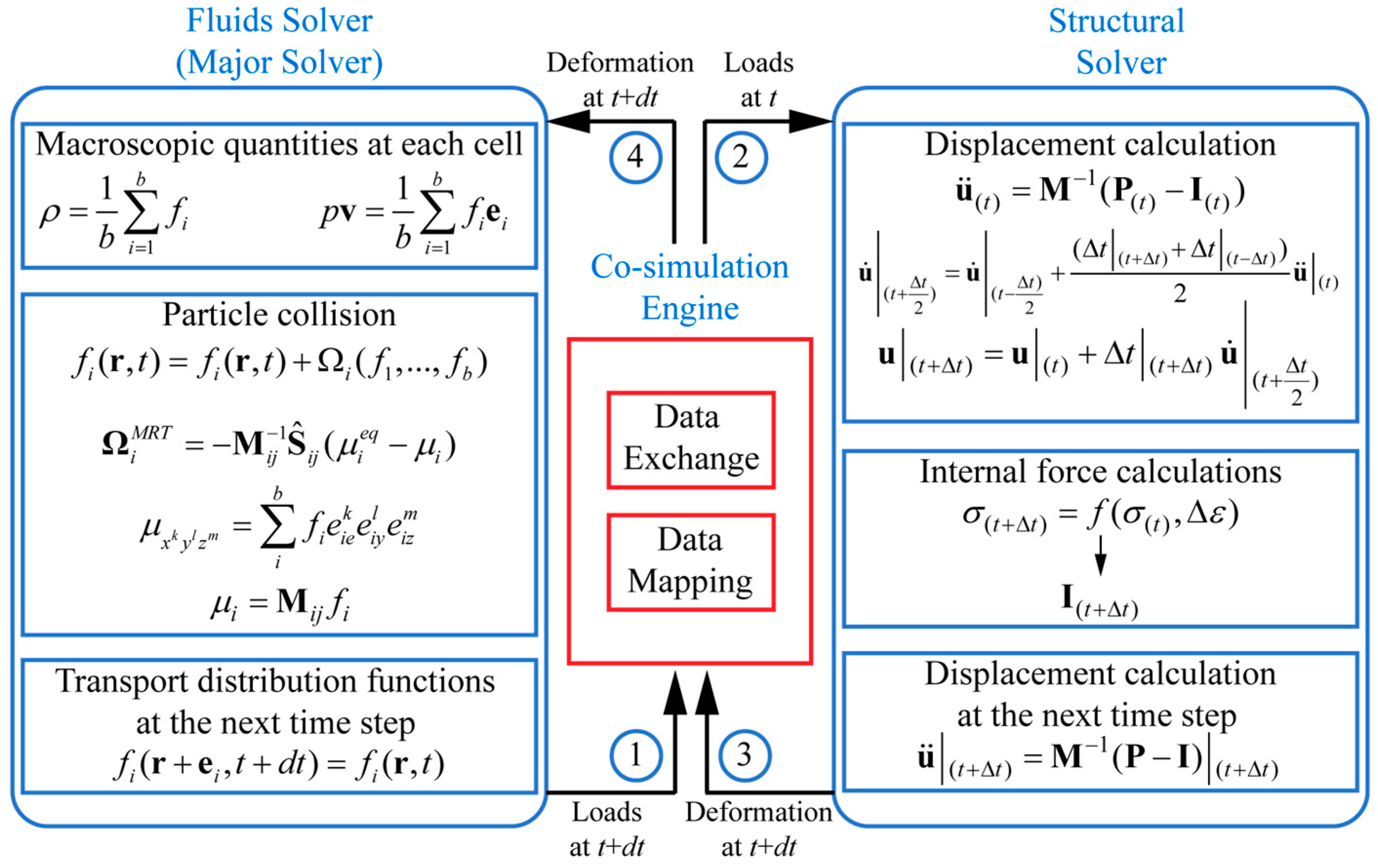
To facilitate the data interchange between the fluid dynamics solver and the structural dynamics solver, and to achieve fluid–structure interactions (FSIs), the Abaqus Co-Simulation Engine (CSE) is deployed to orchestrate the linkage between XFlow and Abaqus/Explicit. The Abaqus CSE oversees the coupling by facilitating data transfer between the solvers and aligning data on the fluid–structure interface grid. In this research, the Abaqus CSE synchronizes the solvers in real-time, utilizing the explicit Gauss–Seidel method, which operates sequentially as one field trails the other by a single coupling step. XFlow is designated as the primary solver in the coupling sequence, dictating the time step preference for data exchange as per the Abaqus CSE. This engine facilitates bidirectional FSIs by transferring forces from XFlow to Abaqus/Explicit and structural displacements in the reverse direction. The co-simulation workflow is depicted in a block diagram in Figure 1. Additionally, the CSE’s key feature is data mapping. Given the infeasibility of one-to-one correspondence between the FEA and LBM meshes, the CSE employs a sophisticated and robust interpolation technique to manage this essential task effectively.

2.2. Validation of FSI Method

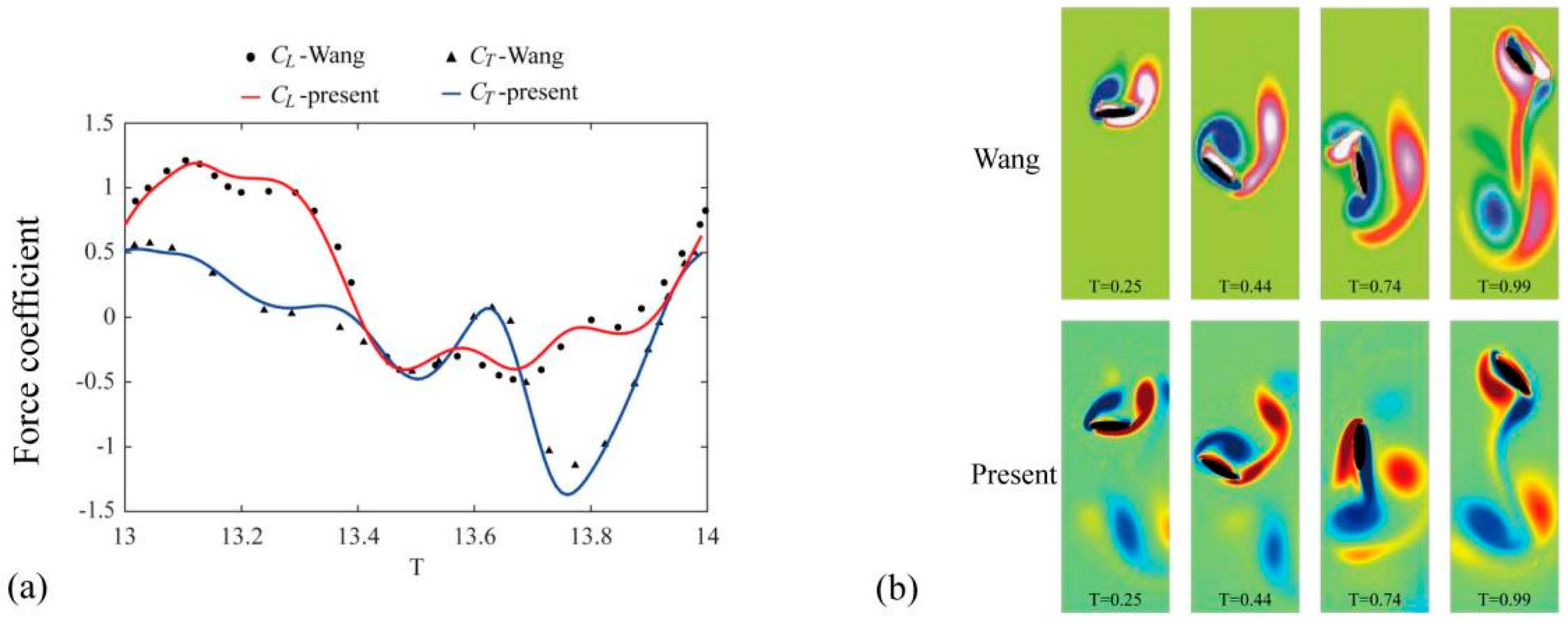
To substantiate the accuracy of the numerical approach presented, we scrutinize the characteristic flow patterns associated with the motion of flapping wings. As depicted in Figure 2a, the temporal variations in the horizontal and vertical force coefficients during the fourteenth wingbeat of a hovering dragonfly are illustrated, aligning with the analysis conducted by Wang [18]. The aerodynamic forces derived from the simulation method outlined in this study are found to closely match the referenced results. Figure 2b presents a comparative analysis of the vortex contours for the flapping wing. Observations indicate that the flow fields near the wing by this numerical approach align well with Wang’s methodology, with an enhanced depiction and capturing of the vortex wake.

2.3. Geometric Model

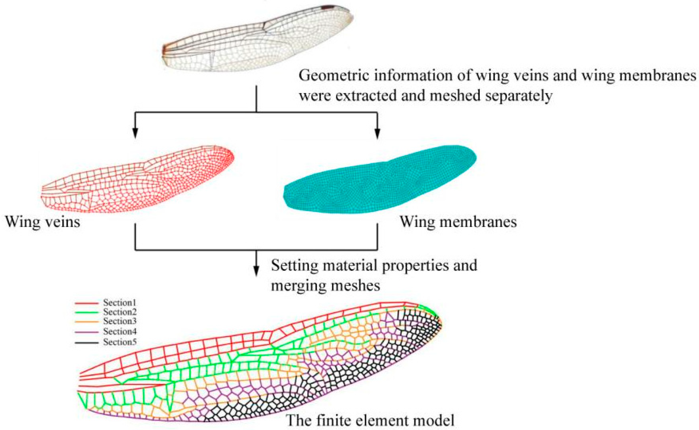
To simulate the flow field of a dragonfly forewing flapping, a model of the dragonfly wing is first constructed. In order to obtain accurate geometric information on dragonfly wings, the digitized images of dragonfly wings were analyzed with Imageware software to extract the geometric layout of the veins and the membrane structure. Subsequently, the geometric details of the wings were imported into Abaqus for the purpose of constructing the model. The membrane structure of such a wing is a naturally occurring biopolymer membrane primarily composed of structural proteins [19,20], with the thickness varying between 5 and 10 μm and gradually thinning from the leading to trailing edge [21]. Therefore, the four-node finite-membrane-strain shell element S4R, with a thickness of 5 µm, was selected to simulate the wing membrane. The primary supporting structure within a dragonfly’s wing vein is the chitinous layer. Hence, the wing vein can be simplified into hollow tube elements [22,23], which are simulated using the two-node Lagrangian interpolated beam cell B31. Based on biological measurements [24,25], the wings were divided into five sections according to the diameter of the wing veins, as shown in Figure 3.

Table 1. The parameter settings of the structural characteristics.

Vein Region	Material	Outer Diameter (μm)
1	E = 4 × 1011 Pa ρ = 1200 kg/m3 γ = 0.3	135
2		100
3		85
4		70
5		55
Membrane	Material	Thickness (μm)
	E = 3.75 × 109 Pa ρ = 1200 kg/m3 γ = 0.3	5

illustrates the material characteristics of both the veins and the membrane across each section.

In real flight, dragonflies use the muscles in their thorax and abdomen to drive their wings to flap. Hence, it is necessary to apply restraints at the wing’s base in the finite element model. The wing’s movement can be comprehensively specified by establishing the motion equations, which incorporate six degrees of freedom for the nodes at the wing’s base. The kinematics of the wing are referenced from the motion of the forewings during dragonfly hovering flight [26].

3. Results and Analysis

3.1. Aerodynamics Force

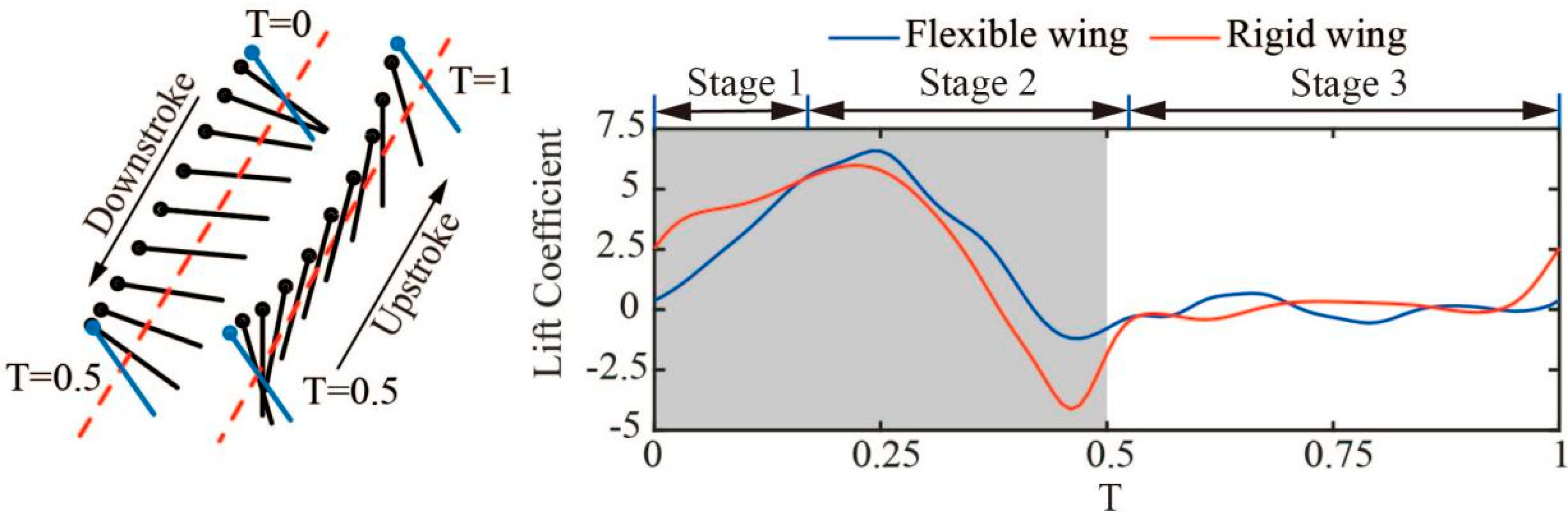
This part of the analysis examines the variation in lift forces over time for both flexible and rigid wings during their flapping motion. The flexible wing’s finite element model was outlined in Section 2.3, whereas the rigid wing model is treated as an inflexible entity. Due to the abrupt changes in the flow field during the transition of the wing from rest to flap, there is a discontinuity in lift. Therefore, the force data from the first three flapping cycles are discarded, and lift data from the fourth to sixth flapping cycles with good periodicity were selected for time averaging.

Figure 4 presents a comparison of the lift forces produced by both flexible and rigid wings under identical flapping motion parameters. It can be observed that, within a complete cycle, the influence of flexible deformation on lift can be divided into three stages: Phase 1(T = 0~0.15), where the lift of the rigid wing is greater than that of the flexible wing; Phase 2 (T = 0.15~0.55), where flexible deformation contributes to an increase in lift; Phase 3 (T = 0.55~1.0) (i.e., the upstroke phase), where the lift force by a flexible wing is typically similar to that of a rigid wing.

The mean lift coefficients over a complete cycle for the flexible wing and rigid wing are 1.51 and 1.40, respectively, indicating a lift gain of 7.86% for flexible wings.

3.2. Flexible Deformation and Flow Fields of Flapping Wing

From the analysis presented in Section 3.1, it is clear that the flexible wing outperforms the rigid wing in terms of lift during the mid-downstroke. To gain a better understanding of the aerodynamic principles behind the increased lift of the flexible wing, the paper investigates the flow field at different sections along the wingspan of both wing types at the midpoint of the downstroke (T = 0.25).

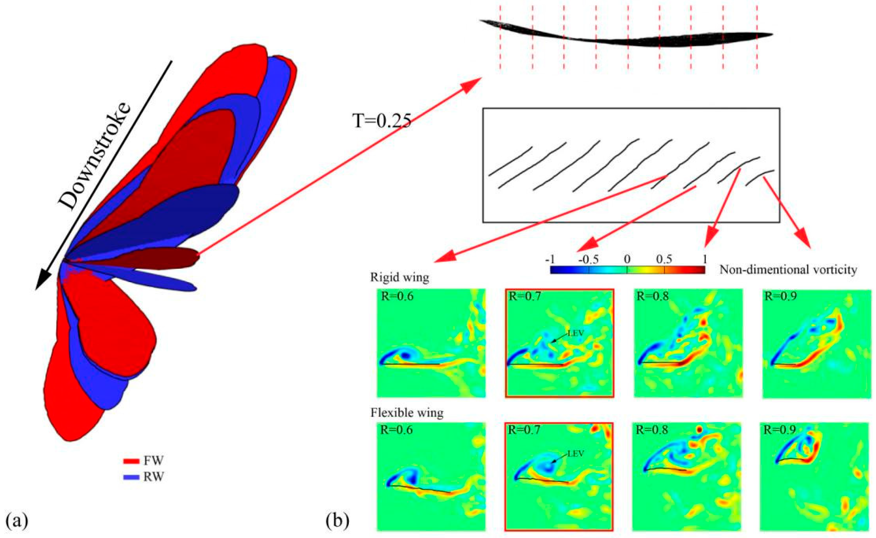
Figure 5a illustrates the geometrical differences between the FW (flexible wing) and RW (rigid wing) throughout the downstroke phase. Influenced by aerodynamic force and inertial effects, the FW exhibits significant deformation.

Figure 5b presents the spanwise two-dimensional flow fields ranging from 0.1R to 0.9R starting from the wing root extending to the wing tip (where R denotes the total wing length) at T = 0.25. The data indicate that, in the proximity of the wing root (R < 0.6), the 2D flow patterns for both the flexible and rigid wings at equivalent spanwise locations are nearly identical, rendering the impact of wing flexibility negligible. Nonetheless, beyond R = 0.6, the influence of flexible deformation on flow structure stability becomes pronounced. To delve deeper into the aerodynamic implications of flexible deformation near the wingtip, the contours of dimensionless vorticity and dimensionless pressure were extracted, and they presented within a range of 0.6R to 0.9R.

In the case of the rigid wing, as the vortex formation progresses from 0.6R to 0.9R, the integrity of the leading-edge vortex (LEV) structure starts to deteriorate. The LEV, which is the primary contributor to lift, is created at the wing’s leading edge during the flapping motion. In contrast, the flexible wing maintains a stable vortex structure closer to the wingtip. Observing at R = 0.7, it is evident that the LEV of the rigid wing has begun to disintegrate, whereas the flexible wing’s LEV sustains its stability. The stability of the LEV structure is crucial for lift generation, which accounts for the enhanced lift of the flexible wing observed during the mid-downstroke phase.

4. Discussion and Conclusions

This study introduces an efficient and precise fluid–structure interaction (FSI) simulation technique utilizing the Lattice Boltzmann Method (LBM) that is tailored for the dynamic analysis of anisotropic and intricate models undergoing significant deformation. A finite element model that reflects the structural resilience of a dragonfly’s wing is developed to explore the aerodynamic impacts of flexible wing deformation during flapping maneuvers through FSI simulation. The findings reveal that the average lift coefficients over a cycle for the flexible and rigid wings are 1.51 and 1.40, respectively, indicating a 7.86% increase in lift efficiency for the flexible wing.

To elucidate the enhanced lift performance of the flexible wing, a comparison of the wing deformation and flow fields between the flexible and rigid wings is conducted. It is observed that, during the mid-downstroke phase, the flexible wing’s deformation results in a chordwise curvature, which helps maintain the stability of the leading-edge vortex (LEV) structure, thereby contributing to increased lift.

The reliability and accuracy of the present FSI method for simulating large deformation motions of anisotropic models (e.g., the flexible wing of MAVs) are verified by simulating the flexible-wing flapping of dragonflies.

References

- Bomphrey, R.J.; Nakata, T.; Phillips, N.; Walker, S.M. Smart wing rotation and trailing-edge vortices enable high frequency mosquito flight. Nature 2017, 544, 92–95. [Google Scholar] [CrossRef]
- Hefler, C.; Noda, R.; Qiu, H.H.; Shyy, W. Aerodynamic performance of a free-flying dragonfly-A span-resolved investigation. Phys. Fluids 2020, 32, 041903. [Google Scholar] [CrossRef]
- Kasoju, V.T.; Santhanakrishnan, A. Aerodynamic interaction of bristled wing pairs in fling. Phys. Fluids 2021, 33, 031901. [Google Scholar] [CrossRef]
- Nakata, T.; Phillips, N.; Simoes, P.; Russell, I.J.; Cheney, J.A.; Walker, S.M.; Bomphrey, R.J. Aerodynamic imaging by mosquitoes inspires a surface detector for autonomous flying vehicles. Science 2020, 368, 634–637. [Google Scholar] [CrossRef] [PubMed]
- Zhang, J.D.; Huang, W.X. On the role of vortical structures in aerodynamic performance of a hovering mosquito. Phys. Fluids 2019, 31, 051906. [Google Scholar] [CrossRef]
- Zhou, C.; Wu, J.H. Kinematics, Deformation, and Aerodynamics of a Flexible Flapping Rotary Wing in Hovering Flight. J. Bionic Eng. 2021, 18, 197–209. [Google Scholar] [CrossRef]
- Cheng, X.; Sun, M. Wing kinematics and aerodynamic forces in miniature insect Encarsia formosa in forward flight. Phys. Fluids 2021, 33, 021905. [Google Scholar] [CrossRef]
- Dudley, T.R. Mechanics of Forward Flight in Insects. Ph.D. Thesis, University of Cambridge, Cambridge, UK, 1987. [Google Scholar]
- Ellington, C.P. The Aerodynamics of Hovering Insect Flight. III. Kinematics. Philos. Trans. R. Soc. Lond. B Biol. Sci. 1984, 305, 41–78. [Google Scholar]
- Ennos, R. The Kinematics and Aerodynamics of the Free Flight of some Diptera. J. Exp. Biol. 1989, 142, 49–85. [Google Scholar] [CrossRef]
- Li, C.; Dong, H. Wing kinematics measurement and aerodynamics of a dragonfly in turning flight. Bioinspiration Biomim. 2017, 12, 026001. [Google Scholar] [CrossRef]
- Rajabi, H.; Ghoroubi, N.; Darvizeh, A.; Appel, E.; Gorb, S.N. Effects of multiple vein microjoints on the mechanical behaviour of dragonfly wings: Numerical modelling. R. Soc. Open Sci. 2016, 3, 150610. [Google Scholar] [CrossRef] [PubMed]
- Rajabi, H.; Ghoroubi, N.; Malaki, M.; Darvizeh, A.; Gorb, S.N. Basal Complex and Basal Venation of Odonata Wings: Structural Diversity and Potential Role in the Wing Deformation. PLoS ONE 2016, 11, e0160610. [Google Scholar] [CrossRef] [PubMed]
- Walker, S.M.; Thomas, A.L.R.; Taylor, G.K. Deformable wing kinematics in free-flying hoverflies. J. R. Soc. Interface 2010, 7, 131–142. [Google Scholar] [CrossRef] [PubMed]
- Wang, H.; Zeng, L.J.; Yin, C.Y. Measuring the body position, attitude and wing deformation of a free-flight dragonfly by combining a comb fringe pattern with sign points on the wing. Meas. Sci. Technol. 2002, 13, 903–908. [Google Scholar] [CrossRef]
- Peng, L.S.; Zheng, M.Z.; Pan, T.Y.; Su, G.T.; Li, Q.S. Tandem-wing interactions on aerodynamic performance inspired by dragonfly hovering. R. Soc. Open Sci. 2021, 8, 202275. [Google Scholar] [CrossRef] [PubMed]
- Peng, L.; Pan, T.; Zheng, M.; Song, S.; Su, G.; Li, Q. Kinematics and Aerodynamics of Dragonflies (Pantala flavescens, Libellulidae) in Climbing Flight. Front. Bioeng. Biotechnol. 2022, 10, 795063. [Google Scholar] [CrossRef] [PubMed]
- Wang, Z.J. Two dimensional mechanism for insect hovering. Phys. Rev. Lett. 2000, 85, 2216–2219. [Google Scholar] [CrossRef]
- Wootton, R.J. Functional Morphology of Insect Wings. Annu. Rev. Entomol. 1992, 37, 113–140. [Google Scholar] [CrossRef]
- Combes, S.A.; Daniel, T.L. Flexural stiffness in insect wings I. Scaling and the influence of wing venation. J. Exp. Biol. 2003, 206, 2979–2987. [Google Scholar] [CrossRef]
- Ren, H.H.; Wang, X.S.; Li, X.D.; Chen, Y.L. Effects of Dragonfly Wing Structure on the Dynamic Performances. J. Bionic Eng. 2013, 10, 28–38. [Google Scholar] [CrossRef]
- Darvizeh, M.; Darvizeh, A.; Rajabi, H.; Rezaei, A. Free vibration analysis of dragonfly wings using finite element method. Int. J. Multiphysics 2009, 3, 101–110. [Google Scholar] [CrossRef]
- Jongerius, S.R.; Lentink, D. Structural Analysis of a Dragonfly Wing. Exp. Mech. 2010, 50, 1323–1334. [Google Scholar] [CrossRef]
- Wainwright, S.A.; Biggs, W.D.; Currey, J.D.; Gosline, J.M. Mechanical Design in Organisms; Princeton University Press: Princeton, NJ, USA, 1982. [Google Scholar]
- Vincent, J.; Wegst, U. Design and mechanical properties of insect cuticle. Arthropod Struct. Dev. 2004, 33, 187–199. [Google Scholar] [CrossRef] [PubMed]
- Norberg, R. Hovering Flight of the Dragonfly Aeschna juncea L., Kinematics and Aerodynamics. In Swimming and Flying in Nature; Wu, T.Y., Brennen, C.J.B.C., Eds.; Plenum Press: New York, NY, USA, 1975; pp. 763–781. [Google Scholar]