Review of Vehicle Motion Planning and Control Techniques to Reproduce Human-like Curve-Driving Behavior ^†

Abstract

Among the many technological challenges of automated driving development, there is an increasing focus on the behavior of these systems. Behavior is usually associated with multiple layers of control. In this paper, we focus on motion planning and control, and how these layers can be tailored to produce different behavior. Our review aims to collect and judge the most used techniques in the field of path planning and control. It has been revealed that model predictive planning and control provides high flexibility, with the cost of high computational capacity. There are simpler algorithms, such as pure-pursuit and Stanley controllers, however, these have very few parameters, therefore, the number of possible behavior patterns is limited.

1. Introduction

In the field of Advanced Driver Assistance Systems (ADAS), one of the most widely used functions is the Lane Keep or Lane Centering System (LKS or LCS) [1]. This function monitors the drivable corridor and keeps the vehicle in the center of the lane. To do that, the path-planning module calculates a reference line, which is then handed over to the vehicle controller. Even though there are many path-planning algorithms in the field [2,3,4,5,6,7,8,9], in a lot of cases, the reference line is associated with the centerline of the lane. Then, the controller—based on its internal policy—calculates a target steering angle, which is then applied to the actuator controls. In the end, the vehicle’s lateral motion is influenced by actuating the steering wheel. The composition of path planning and control is a commonly accepted technique of building automated driving systems [10]. Different behavior patterns can be recognized by tuning the control algorithm’s free parameters. In the literature, there are control algorithms that can be classified into one of the following three types:

• Inverse-dynamic models;
• Compensatory models;
• Feedforward models.

Inverse-dynamic models use a vehicle model to calculate the target steering angle to reach a certain target state (i.e., vehicle position). Such controllers are the pure-pursuit algorithm [11] or the Stanley controller [12]. Compensatory models assume that drivers intervene in relation to the error of a certain output quantity, such as the vehicle position or orientation. Hence, these control models often act as closed-loop controllers, and the drivers are modeled using simple PID or other linear control structures [13,14,15,16]. Feedforward models also use a vehicle model to predict its behavior on a certain input trajectory. Then, based on a pre-defined objective function, they optimize the behavior and calculate the optimum input trajectory on a so-called preview horizon. Such controllers are the model predictive controls [17,18,19,20]. In this paper, we implement algorithms of each type in MATLAB and run a closed-loop simulation on a real-world road segment. We compare each algorithm by its ability to provide accuracy and flexible paths and its computation effort.

2. Materials and Methods

2.1. Methods

The model is a kinematic single-track model. The model equations are given in Equation (1), where $T_s$ is the sampling time, $L$ is the axis distance of the vehicle, ${\mathit{x}}_k={\left[x y \mathsf{\Theta }\right]}^T$ is the state vector, and $u_k={\alpha }_k$ is the input of the system. The used coordinate frame $\left(x,y\right)$, the local frame $(\xi ,\eta )$, and the related kinematic quantities are shown in Figure 1a. Finally, the output vector is ${\mathit{y}}_k={\left[y_k {\mathsf{\Theta }}_k\right]}^T$.

$$f=\left[\begin{array}{c}{x}_k\\ y_k\\ {\mathsf{\Theta }}_k\end{array}\right]=x_k=\left[\begin{array}{c}{x}_{k-1}+T_s{v}_{\xi }\cos \left({\Theta }_{k-1}\right)\\ y_{k-1}+T_s{v}_{\xi }\sin \left({\Theta }_{k-1}\right)\\ {\mathsf{\Theta }}_{k-1}+{\displaystyle \frac{T_s{v}_{\xi }\tan \left({\alpha }_f\right)}{L}}\end{array}\right]$$

(1)

The kinematic single-track model is implemented in MATLAB. The simulations are run using a real-life road section from Hungary, Road 31. The path is shown in Figure 2. The model given in Equation (1) is implemented in MATLAB, too.

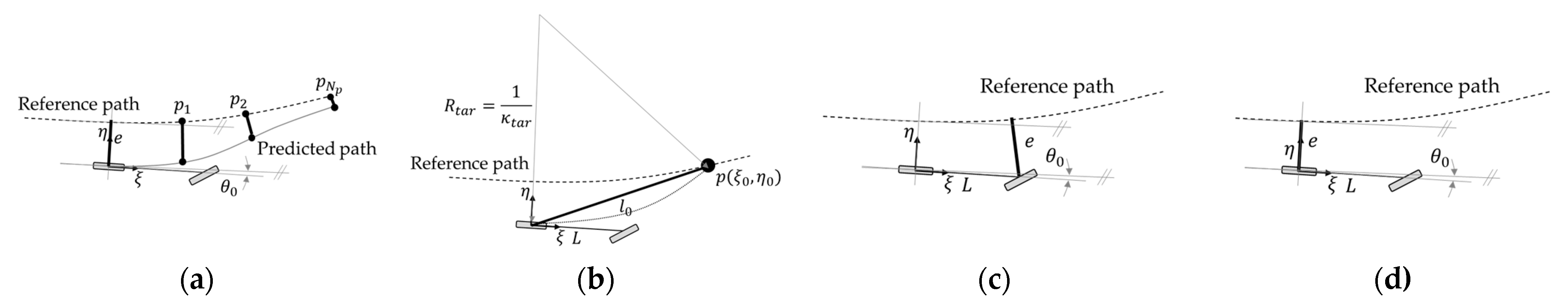
2.2. Model Predictive Control

The MPC algorithms rely on the following basic steps:

• Prediction of the vehicle states $X_k=[x_k{x}_{k+1}\dots x_{k+N_p-1}]\in {\mathbb{R}}^{n\times N_p}$, $X_k=f(X_{k-1},U,)$, given the input vector $U=[u_k{u}_{k+1}\dots u_{k+N_p-1}]\in {\mathbb{R}}^{m\times N_p}$ on the prediction horizon $N_p$, and the output $Y=[y_k{y}_{k+1}\dots y_{k+N_p-1}]\in {\mathbb{R}}^{o\times N_p}$, where $o$ is the number of outputs;
• Calculating the reference output, given the prior path $Y_{ref}=g(\gamma \left(p_{driver}\right),v_{\xi }, N_p, T_h)$, where $T_h$ is the prediction horizon and $\gamma$ is the representation of the prior path;
• Calculating the cost $h(Y, Y_{ref},Y_{traffic}, w_{driver},c_{driver})$.

The optimization variables are elements of $U$, and the cost function $h(·)$ is minimized as follows:

$$\begin{gathered} \underset{U}{\min }h(·) \\ s.t.u_{min}\le U\le u_{max} \end{gathered}$$

As model Equation (1) is non-linear, a numerical non-linear optimization algorithm is used. This is carried out in MATLAB, using the ‘fmincon’ function of the optimization toolbox. The initial value of the input vector $U$ is zero, then, the previously calculated optimal input is taken as the initial point of the next optimization loop. The MPC cost function always includes a term that is associated with the error of the output(s) to the reference. Thus, the reference output vector $y_{ref}$ is calculated from the prior path and interpolated to the predicted vehicle positions in Equation (2), as follows:

$$Y_{ref}=interp(\gamma ,x_{pred}),$$

(2)

where $x_{pred}=x_0+[d{x}_{1}d{x}_2\dots d{x}_k\dots d{x}_{N_p}]$, $d{x}_k=v_{\xi }\mathrm{c}\mathrm{o}\mathrm{s}\left({\mathsf{\Theta }}_k\right)$, and $x_0$ is the vehicle position at the time of planning. The geometric relations are shown in Figure 3a. The cost function also includes a term that is controversial with the output error, namely the amplitude of the steering angle. Then, the final cost function is given by Equation (3), as follows:

$$h\left(·\right)=\sum _{i=1}^{N_p}{\left(y_{ref,i}-y_i\right)}^T{W}_y\left(y_{ref,i}-y_i\right)+u_i^2{w}_{\alpha },$$

(3)

where $W_y=diag\left(\left[w_{dy} w_{d\Theta }\right]\right)$ is the weight matrix, $w_{\alpha }$ is the input weight, and $y_{ref,i}=Y[:,i]$, i.e., the $i^{th}$ column of the output matrix.

2.3. Pure-Pursuit Controller

The pure-pursuit controller relies on a simple concept. A look-ahead point is calculated, and then a circular path is defined, which leads the vehicle from its location to this look-ahead point. Geometrical relations are shown in Figure 3b. The curvature of the target path is calculated according to Equation (4), as follows:

$${\kappa }_{tar}={\displaystyle \frac{l_0^2}{2{\eta }_0}}$$

(4)

Then, the target steering angle can be calculated according to Equation (4). The algorithm has one parameter $l_0$, which also defines $p_0({\xi }_0,{\eta }_0)$. Often—to overcome speed dependency issues—the look-ahead distance $l_0$ is replaced by look-ahead time, and then $l_0=v_{\xi }{t}_0$.

2.4. Stanley Controller

The Stanley controller is a simple but robust way of leading vehicles. There are two main differences compared to the pure-pursuit algorithm, as follows: the deviation from the reference path (often called cross-track error) is calculated for the front axis of the vehicle. Secondly, the orientation error to the tangent of the reference line at the vehicle position is also considered. Its illustration is shown in Figure 3c. Then, the target steering angle can be calculated according to Equation (5). It has one parameter, which is the Stanley coefficient $k$.

$${\alpha }_{tar}=\mathrm{atan}\left({\displaystyle \frac{ke}{v_{\xi }}}\right)+{\theta }_0$$

(5)

2.5. Compensatory Driver Model

The compensatory driver model in this implementation is a parallel PID controller, which considers the deviation from the reference path and its integral and derivative terms [13]. Its geometrical relations are shown in Figure 3d. The error quantities are calculated at the vehicle position. The target steering angle is given by Equation (6). The algorithm has 3 parameters, and the control coefficients are associated with the different terms.

$${\alpha }_{tar}=Pe+I\int edt+D{\displaystyle \frac{de}{dt}}$$

(6)

3. Results

3.1. Evaluation Criteria

In Section 3.2, the experiments are presented to show the behavior of each algorithm. The following quantities are examined:

• $\delta \left(t\right)$—lane offset to the centerline;
• ${\alpha }_f$—front road wheel angle, which is the input of the system;
• $t_{ct}$—computational time/simulation cycle, measured in MATLAB.

The results are generated using the simulation framework detailed in Section 2.1.

3.2. Experiments

The following tests are run to show the working principle of the proposed planning and control algorithm:

• Test I: Neutral behavior, which is the compromise between the steering wheel oscillation and the tracking accuracy;
• Test II: Mistune—to produce a behavior that deviates from the neutral behavior.

The parameters of each test case are given in

Table 1. Parameters and description of the test cases.

	MPC	Pure-Pursuit	Stanley	PID
Test I.	$w_{dy}=0.0$$, w_{d\Theta }=2.0$$, w_{\alpha }=1.0$	$t_0=1.5 \mathrm{s}$	$k=1$	$P=0.1$$, I=0.01, D=0.05$
Test II.	$w_{dy}=0.0$$, w_{d\Theta }=2.0$$, w_{\alpha }=1.5$	$t_0=2.25 \mathrm{s}$	$k=0.5$	$P=0.01$$, I=0.01$$, D=0.05$

.

The results of Test I are shown in Figure 4. The MPC algorithm has the highest computational capacity needs, while providing moderate error on the position output. The steering angle has low frequency oscillation. The pure-pursuit algorithm provides a moderate error on the position output but a very smooth steering angle. Its computational time need is the lowest. The Stanley controller provides the best track error; however, the steering angle has high frequency oscillation. The simple PID controller produces a very similar output as the Stanley controller, with both having higher computational time needs than pure-pursuit. Interestingly, all of the controllers result in overshoot in the curves, except pure-pursuit, which cuts the curve slightly.

A second test was run, where each controller was tuned differently. The aim was to show how the parameters influence the output behavior. The results are shown in Figure 5. Having a higher weight associated with the input signal, the output error from the NMPC algorithm increases. Having a higher look-ahead time, the pure-pursuit algorithm cuts the curves more significantly, which is also a usual behavior of drivers. It must be noted that this algorithm is not suitable to use for outer-lane driving in curves. Having a lower Stanley coefficient results in higher deviation from the reference path and causes increased computational time at certain parts of the simulation. However, the steering angle does not change significantly. Having lower proportional gain, the PID controller results in a much higher overshoot in curves, while not significantly changing the input steering angle. Interestingly, similarly to the Stanley controller, the computational time increases in this case as well.

4. Conclusions

4.1. Contribution

In this paper, we have implemented prototypically and compared the most relevant control algorithms. It has been shown that, considering a simple kinematic bicycle model, the MPC algorithm produces the worst output. However, it is also emphasized that the advantages of MPC come when the complexity of the system under control grows. Also, other terms can be added to the objective function (e.g., traffic, distance to lane edges, etc.), which increases the flexibility of this algorithm. Pure-pursuit provides the smoothest steering angle signal, however, its flexibility to provide different motion behavior is low. It can only produce curve cuts. Stanley and PID controllers are highly similar, however, while the Stanley controller is relatively ineffective on the parameter changes, the PID controller performance degraded a lot when changing the gains.

4.2. Limitations

The implementation took place in MATLAB, considering only a kinematic single-track model. This makes the value of the work lower, as the results cannot be directly taken over to practical implementation, e.g., in real-vehicle controllers. Also, the tuning was carried out empirically, which makes the comparison less reliable. However, the characteristics of the controllers could be nicely shown.

4.3. Outlook

In the future, we plan to continue the analysis with real-vehicle application, as well as further extension of the MPC algorithm, to show the real features of these controllers in terms of human-like driving of automated systems.

References

1. United Nations. Economic and Social Council: Proposal for a new UN Regulation on uniform provisions concerning the approval of vehicles with regards to Automated Lane Keeping System. In Proceedings of the ECE/TRANS/WP.29/2020/81, Geneva, Switzerland, 23–25 June 2020. [Google Scholar]
2. Werling, M.; Ziegler, J.; Kammel, S.; Thrun, S. Optimal trajectory generation for dynamic street scenarios in a Frenét frame. In Proceedings of the 2010 IEEE International Conference on Robotics and Automation, Anchorage, AK, USA, 3–7 May 2010; pp. 987–993. [Google Scholar]
3. Osa, T. Multimodal trajectory optimization for motion planning. Int. J. Robot. Res. 2020, 39, 983–1001. [Google Scholar] [CrossRef]
4. Li, A.; Jiang, H.; Li, Z.; Zhou, J.; Zhou, X. Human-like trajectory planning on curved road: Learning from human drivers. IEEE Trans. Intell. Transp. Syst. 2020, 21, 3388–3397. [Google Scholar] [CrossRef]
5. Yu, C.; Ni, A.; Luo, J.; Wang, J.; Zhang, C.; Chen, Q.; Tu, Y. A novel dynamic lane-changing trajectory planning model for automated vehicles based on reinforcement learning. J. Adv. Transp. 2022, 2022, 8351543. [Google Scholar] [CrossRef]
6. Zhang, J.; Chen, H.; Song, S.; Hu, F. Reinforcement learning-based motion planning for automatic parking system. IEEE Access 2020, 8, 154485–154486. [Google Scholar] [CrossRef]
7. Chen, L.; Jiang, Z.; Cheng, L.; Knoll, A.C.; Zhou, M. Deep reinforcement learning based trajectory planning under uncertain constraints. Front. Neurorobot. 2022, 16, 883562. [Google Scholar] [CrossRef] [PubMed]
8. Yu, S.; Shen, C.; Ersal, T. Nonlinear Model Predictive Planning and Control for High-Speed Autonomous Vehicles on 3D Terrains. IFAC-PapersOnLine 2021, 54, 412–417. [Google Scholar] [CrossRef]
9. Eilbrecht, J.; Bieshaar, M.; Zernetsch, S.; Doll, K.; Sick, B.; Stursberg, O. Model-Predictive Planning for Autonomous Vehicles Anticipating Intentions of Vulnerable Road Users by Artificial Neural Networks. In Proceedings of the IEEE Symposium Series on Computational Intelligence (SSCI), Honolulu, HI, USA, 27 November–1 December 2017. [Google Scholar]
10. Peters, B.; Nilsson, L. Modelling the driver in control. In Modelling Driver Behaviour in Automotive Environments; Springer: London, UK, 2007; pp. 85–104. [Google Scholar]
11. Coulter, R.C. Implementation of the Pure Pursuit Path Tracking Algorithm; Carnegie Mellon University, Robotics Institute: Pittsburgh, PA, USA, 1992. [Google Scholar]
12. Hoffmann, G.M.; Tomlin, C.J.; Montemerlo, M.; Thrun, S. Autonomous Automobile Trajectory Tracking for Off-Road Driving: Controller Design, Experimental Validation and Racing. In Proceeding of the American Control Conference, New York, NY, USA, 9–13 July 2007. [Google Scholar]
13. Rathgeber, C.; Winkler, F.; Odenthal, D.; Müller, S. Lateral trajectory tracking control for autonomous vehicles. In Proceedings of the European Control Conference (ECC), Strasbourg, France, 24–27 June 2014. [Google Scholar]
14. Salvucci, D.D.; Gray, R. A two-point visual control model of steering. Perception 2004, 33, 1233–1248. [Google Scholar] [CrossRef] [PubMed]
15. Ungoren, A.Y.; Peng, H. An Adaptive Lateral Preview Driver Model. Veh. Syst. Dyn. 2005, 43, 245–259. [Google Scholar] [CrossRef]
16. Hess, R.A.; Modjtahedzadeh, A. A control theoretic model of driver steering behavior. IEEE Control Syst. Mag. 1990, 10, 3–8. [Google Scholar] [CrossRef]
17. McAdam, C.C. An Optimal Preview Control for Linear Systems. J. Dyn. Syst. Meas. Control 1980, 1, 188–190. [Google Scholar] [CrossRef]
18. Morari, M.; Garcia, C.E.; Prett, D.M. Model Predictive Control: Theory and practice. In Proceedings of the IFAC Model Based Process Control, Atlanta, GA, USA, 13–14 June 1988. [Google Scholar]
19. Katriniok, A.; Maschuw, J.P.; Christen, F.; Eckstein, L.; Abel, D. Optimal vehicle dynamics control for combined longitudinal and lateral autonomous vehicle guidance. In Proceedings of European Control Conference, Zürich, Switzerland, 17–19 July 2013. [Google Scholar]
20. Jiang, H.; Tian, H.; Hua, Y. Model predictive driver model considering the steering characteristics of the skilled drivers. Adv. Mech. Eng. 2019, 11, 1687814019829337. [Google Scholar] [CrossRef]
Figure 1. (a) Vehicle quantities and relation to the road centerline; (b) Coordinate system and related quantities of the single-track model.
Engproc 79 00020 g001
Figure 2. Road segment from Road 31, Hungary, used for simulations.
Engproc 79 00020 g002
Figure 3. Schematic representation of each control algorithm. (a) NMPC, where the vehicle motion is predicted on a selected horizon and the right steering angle trajectory is obtained via optimization; (b) Pure-pursuit, where the steering angle target value is directly calculated from a look-ahead point; (c) Stanley controller, which considers both position and angle error of the front axle; (d) PID controller, which follows the generic closed-loop control idea.
Engproc 79 00020 g003
Figure 4. Results of experimental Test I. (a) NMPC, where the computational time is the highest, but the control error is low; (b) Pure-pursuit, resulting in smooth steering trajectory, but increased position error; (c) Stanley, having both low error and low computational time; (d) PID control.
Engproc 79 00020 g004
Figure 5. Results of experimental Test II. (a) NMPC, with increased output error; (b) Pure-pursuit, where increased look-ahead time results in more significant curve cutting; (c) Stanley, where less strict control results in higher error but lower computational time; (d) PID control, where decreased proportional gain results in higher error.
Engproc 79 00020 g005