Abstract
Multi-source autonomous navigation-dependable decision making has a crucial impact on the overall performance of navigation systems. To solve the problem of overall system robustness caused by the intelligent-dependable decision making difficulties of navigation systems from different sources, on an unmanned ground vehicle (UGV) as the carrier, a new multi-source fusion algorithm based on cost function is proposed in this paper. The algorithm uses INS/GNSS/UWB as the sensor data source and is solved by using error-state Kalman filter (ESKF)-based kinematic and static multi-source filtering. After the RSS, positioning residual and positioning stability are selected as parameters and weighted, and the cost function is constructed. The structure of the filtering can be adapted according to the cost function in complex environments. Through mathematical simulation and comparative experiments, the positioning accuracy of the algorithm is improved by 75.9% and 74.44%, respectively, compared to federated filter and traditional ESKF-based kinematic and static filtering. It also improves the reliability, decision-making ability, and robustness of multi-source autonomous navigation system.
1. Introduction
Multi-source autonomous navigation systems in the new generation of national integrated positioning, navigation, and timing (PNT) systems are a key technology for terminal applications such as positioning, navigation, and timing services, and are based on global navigation satellite system (GNSS) navigation as the cornerstone and inertial navigation as the support to meet the needs of the terminal, such as plug-and-play, seamless connection, non-sensitive switching, and trustworthy completeness [1]. Currently, the multi-source autonomous navigation system faces complex and critical system-level information processing decision-making tasks, and the operations of contact, detection, switching, and scheduling of carrier navigation information sources constitute the multi-source autonomous navigation information processing fundamentals. The effects of the decision-making operations directly affect the performance of the multi-source autonomous navigation system [2]. Taking seamless switching scene between indoor and outdoor as an example, GNSS is now mostly used as the main positioning system in outdoor scenes, but due to its weak signal on the ground surface, it is not applicable to indoor scenes [3]. In indoor scenes, ultra-wide band (UWB) with higher overall positioning accuracy is used as the main positioning system. Because of the complex indoor environment, the impact of multipath effect, non-line-of-sight effect, and electronic equipment signal interference caused by environmental factors will result in a reduction in the positioning accuracy of indoor positioning system, and even an inability to locate the situation [4]. Using the angular velocity and specific force information of the carrier relative to the inertial space measured by the inertial measurement unit (IMU), the inertial navigation system (INS) calculates the position, velocity, attitude, and time information of the carrier in the navigation coordinate system through the specific force equation. Although the navigation accuracy of the INS is not easily interfered with by external factors, it cannot be applied to navigation for a long time due to the characteristics of navigation error accumulating with time [5]. Hence, in complex scenarios, if the multi-source autonomous navigation system is unable to make autonomous switching decisions based on the quality of the navigation information sources, the accuracy and robustness of the overall navigation system will be greatly reduced.
In the communication field, switching refers to the process of changing the access point from the current network to another network to ensure the continuity of communication in the process of terminal movement or network access point change. The switching of homogeneous networks is called horizontal switching, and the switching of heterogeneous networks is called vertical switching. Applying this concept to the field of navigation, GNSS is used outdoors and UWB is used indoors, and the working mode of these two systems is not the same, which is a typical heterogeneous network. To connect the services of indoor and outdoor positioning systems, it is necessary to study the switching algorithm between indoor and outdoor positioning systems. Existing indoor and outdoor seamless vertical switching algorithms are mainly classified into RSS-based vertical switching algorithms, fuzzy logic-based vertical switching algorithms, and cost function-based vertical switching algorithms. René Hansen et al. conducted a study on the switching of seamless indoor and outdoor positioning systems, where different switching strategies were analyzed and validated in terms of positioning accuracy and power consumption for both outdoor GPS and indoor WIFI fingerprint positioning systems [6]. Yang et al. also studied the switching of GPS and WIFI, and their focus was on the consideration of the selection of map problem [7]. Deng et al. proposed a switching strategy based on cost function in WSN and WLAN for indoor positioning [8]. The authors of [9] proposed a seamless positioning switching algorithm based on fuzzy logic. In 2015, Wiem et al. conducted further research on fuzzy logic [10]. By analyzing the current status of seamless positioning research, it can be seen that the research on switching is still mainly in the communication field, and the research on the switching between positioning systems is still in the preliminary development stage.
To solve the problem of intelligent autonomous dependable decision making of navigation information in multi-source autonomous navigation under complex scenarios, taking UGV as a carrier, according to the filtering algorithm proposed in the literature [11], combined with the vertical switching algorithm based on the cost function, a cost function-based INS/GNSS/UWB adaptive robust ESKF kinematic and static filtering is proposed in this paper. The cost function of this algorithm was constructed according to the RSS, positioning residuals, and positioning stability factors. The overall filtering structure was adaptively changed through the cost function of the subsystem credibility judgment, and thus achieved the purpose of improving the overall system accuracy and robustness. On this basis, to explore the possibility of the algorithms proposed in this paper in the switching of the trustworthiness of the multi-source autonomous navigation, a simulation experiment of relevant indoor and outdoor scenes was built and carried out in this paper, and the positioning errors were compared with those of the federated filtering algorithm and ESKF-based kinematic and static filtering algorithms, respectively. Through experiments, the suitability of the algorithm for multi-source autonomous navigation-dependable decision making was explored. The experimental results show that the INS/GNSS/UWB adaptive robust ESKF kinematic and static filtering based on the cost function have good robustness, and the filters can be switched to the adaptive structure according to the relevant parameter characteristics of the subsystems, which can provide the filtering basis for the dependable decision making of multi-source autonomous navigation.
2. Kinematic and Static Filtering Based on the ESKF
2.1. ESKF Fundamentals
In most inertial systems today, the ESKF is often preferred to the original state Kalman filtering. ESKF is a typical indirect method of filtering; its prediction and updating processes are directed to the error state of the system, and then the corrected error state is corrected to the system state. Compared to Kalman filtering, the advantages of ESKF include the following: the treatment of rotation, where the state variables can be expressed in terms of minimized parameters; the computational procedure is always near the origin, far from the singularity, and there is no problem of insufficient linearization approximation due to being too far away from the operating point; and the state quantities are small and the second-order variables are relatively negligible. In this paper, two fusion navigation ESKF models are designed in a loosely coupled form, namely, GNSS/INS-based ESKF and UWB/INS-based ESKF, respectively, and the two fusion models are constructed based on the INS-based ESKF model.
2.1.1. ESKF Kinematic Models
In this paper, is adopted as the state vector of the overall system, where represents attitude, velocity, and position, respectively. represents the zero bias of the accelerometer, and represents the zero bias of the gyroscope. In ESKF, the real state vector is as follows:
where represents the nominal state vector and represents the error state vector, , , .
The IMU kinematics model in the ESKF error state, as shown in Equation (2):
where represents the white noise of the acceleration measurements, the zero bias vectors of the acceleration, and represents the white noise of the angular velocity measurements. represents the zero bias vectors of the angular velocity. represents the antisymmetric matrix.
Equation (2) discretization equation can be expressed as follows:
where represents the Gaussian random impulse noise of attitude, represents the Gaussian random impulse noise of velocity, represents the Gaussian random impulse noise with zero bias of acceleration, represents the Gaussian random impulse noise with zero bias of angular velocity, represents the sampling interval, and the corresponding covariance matrix is defined as shown in Equation (4):
where represents the standard deviation of acceleration’s Gaussian white noise, and represents the standard deviation of acceleration zero bias’s Gaussian white noise. represents the standard deviation of angular velocity’s Gaussian white noise, and represents the standard deviation of angular velocity zero bias’s Gaussian white noise. C is a 3 × 3 unit matrix.
2.1.2. ESKF State-Prediction Model
The nominal state vector under discrete conditions is defined as , the error state vector as , the IMU acceleration and angular velocity measurement noise vector as , and the IMU attitude, velocity, acceleration zero bias, and angular velocity zero bias noise vectors as . At moment , the nominal state vector is formulated as follows:
where represents the recursive function of the nominal-state vector. The error-state vector formula for moment is shown in Equation (6):
where represents the recursive function of the error-state vector. The and represent the Jacobi matrices corresponding to the noise-state vector and the error-state vector, respectively. The is the state–transfer matrix from moment to moment . The is the noise–transfer matrix from moment to moment . The specific expressions of and are as shown in Equation (7):
The covariance matrix and error-state vector are as follows in:
where represents the covariance matrix of error-state vector at moment . The represents the state-noise matrix, which is represented as follows:
2.1.3. ESKF Measurement-Prediction Model
In the process of measurement updating, we used the difference in measurement vectors for GNSS and IMU velocity and position as the observation equations for system 1, and the difference in measurement vectors for UWB and IMU velocity and position as the observation equations for system 2. In this paper, the ESKF measurement model is as follows:
where is the measurement vector of the ESKF composed of the INS and system , , and represent the velocity information measured by the INS and system . and represent the position information measured by the INS and system , respectively. The is the measurement design matrix of the ESKF composed of the INS and system . is the measurement noise matrix, where represents velocity’s Gaussian measurement of white noise and represents position’s Gaussian measurement of white noise. The updated equations for the ESKF observation model are as follows:
where is the new interest vector, is the covariance matrix of the new interest vector, is the covariance matrix of the measurement noise, is the Kalman gain matrix, is the estimated vector of error state vectors at the moment , and represents the covariance matrix of .
2.2. Kinematic and Static Filter Structure Based on ESKF
The least squares information sharing principle is used in the federated filter to take full advantage of parallel filtering with multi-source sensors, which has the advantage of a fast solving speed. Due to the fact that both the main and local filters of the federated filtering need to use the same equation of state information, which leads to the correlation between the outputs of the filters, and the fact that the application of the information sharing principle does not take into account this correlation property, the dynamic and static filtering avoids the problem of reusing the carrier equation of state information, which ensures the optimality of the multi-sensor data fusion.
The structure of the kinematic and static filter structure based on ESKF used in this paper is shown in Figure 1. The overall filtering is classified into dynamic ESKF and static ESKF. At any moment the observation calendar element based on the dynamics model of the output of the first system for the kinematic Kalman filter and the state vector obtained by the filtering are zeroed and injected, based on which the navigation information of the rest of the system is added in sequence and the static Kalman filtering is performed. Finally, the injected state vector in the end static filtering is used as the fusion result for all navigation information. The injection process equation is as follows in Equation (12):
where is the vector of true state estimates of the static ESKF, is the vector of nominal state estimates of the static ESKF, and is the vector of error state estimates of the static ESKF.
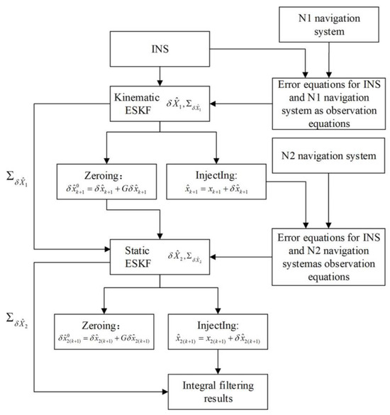
Figure 1.
Structure of ESKF-based kinematic and static filtering.
Meanwhile, after setting the error state vector to zero, the equation is as follows:
where is the static ESKF error state vector after zeroing and is the zeroing design matrix.
3. INS/GNSS/UWB Adaptive Robust ESKF Kinematic and Static Filtering Based on Cost Function
3.1. Switching Algorithm Based on Cost Function
In practice, a single physical quantity such as the RSS is greatly affected by the environment, and the switching effect it characterizes is often not good. At this point, the concept of cost function is introduced, and its core idea is to consider multiple network parameters and assign corresponding weights to these parameters to make the switching as close to the ideal state as possible. The specific formula of the cost function is shown in Equation (14):
where represents the cost function, represents the weight of the parameter, and represents the parameter involved in the operation.
In this paper, three physical quantities, RSS, positioning residuals, and received signal stability, were chosen as evaluation parameters. In switching between positioning systems, the RSS is the most basic reference quantity. For the GNSS system, the signal strength received by the user is relatively stable, so the number of visible stars can be regarded as a different expression of the RSS. For the UWB system, the average RSS value of at least three nodes received is used as the basic reference quantity. The positioning residuals in Kalman filtering can reflect the performance of the positioning system at the current moment, so the positioning residuals are used as the parameter evaluation of the algorithm proposed in this paper. The GNSS signal strength is more stable on the ground, and its stability is relatively high, but the UWB signals are affected by the complex indoor environment, and there will be a large attenuation and jitter, so the stability of the signals of the two systems is also one of the important parameters for evaluating the performance of the system.
Since the same parameter is not standardized in different positioning systems and cannot be used directly for comparison, the collected parameters need to be first normalized before they can be input into the cost function to participate in the calculation. Different parameters are categorized into positive and negative factors according to their contribution value to the system. The normalization function of the positive factor is shown in Equation (15), and the normalization function of the negative factor is shown in Equation (16):
where is the normalized parameter value, is the received parameter value, and and are the maximum and minimum threshold values of the parameter in the system, respectively. In this paper, the RSS and received signal stability were positive factors, and positioning residuals were negative factors.
Due to the different weights of different parameters in the cost function, it is also necessary to assign weights to different parameters. In this paper, based on the judgment matrix of the scalar method used in [12,13], a judgment matrix was established based on the RSS, the positioning residuals, and the received signal stability (Table 1).

Table 1.
The cost function judgment matrix .
The specific procedure for calculating the weight values of each parameter using the factors of the judgment matrix is as follows:
- Normalization: Normalizing each column vector of matrix yields: .
- Summation: Summing by rows gives: .
- Obtaining the power vector: Normalizing to yields a power vector: .
3.2. Integral Filter Structure
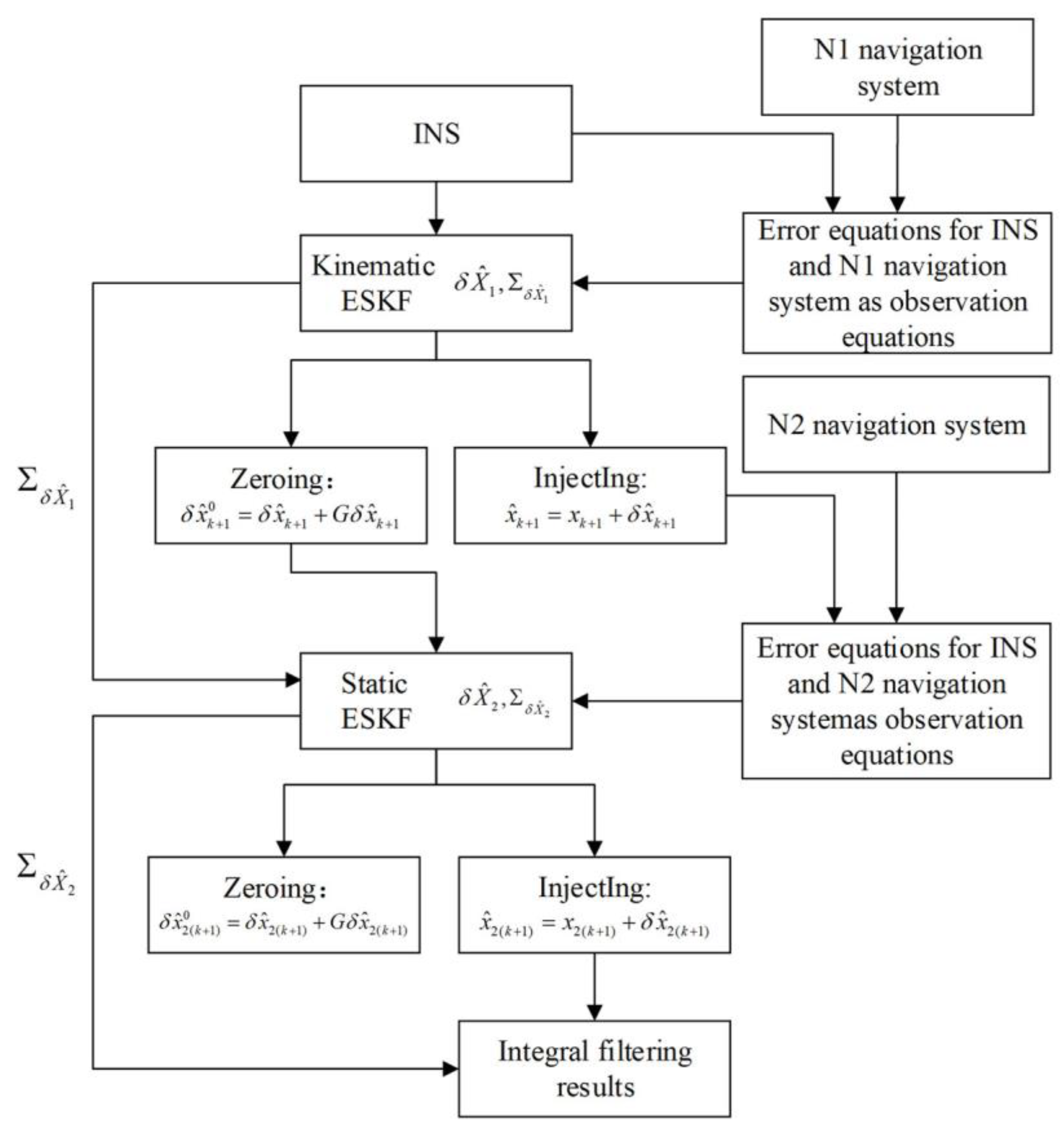
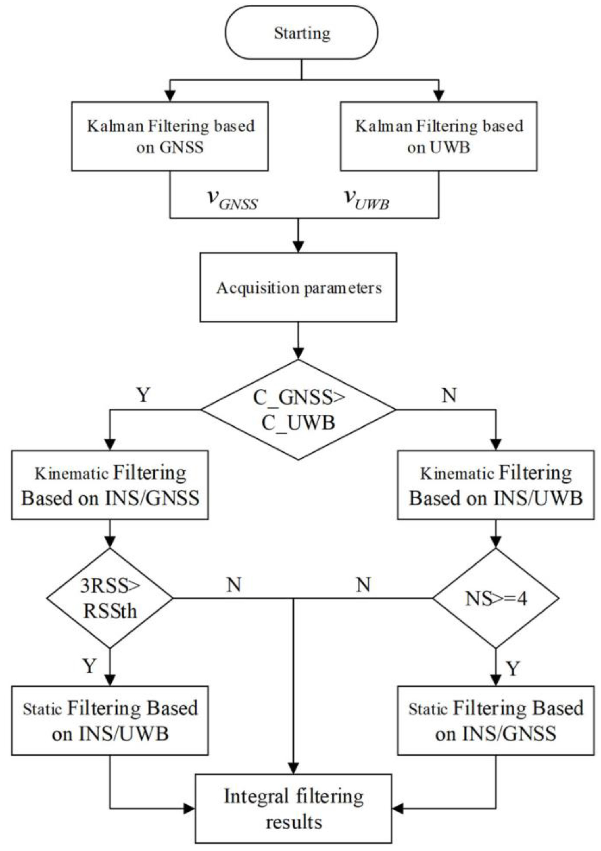
In this paper, the seamless switching scene between indoor and outdoor carried out by the carrier was mainly categorized into outdoor scene, indoor scene, and the transition scene between indoor and outdoor. To improve the trustworthiness and robustness of the fused autonomous navigation system, a new fusion filtering based on INS/GNSS/UWB was designed in this paper. The filtering was based on the kinematic and static filtering of ESKF, through the cost function constructed in the previous section, to judge the environment in which the carrier was located and change the filtering structure autonomously. The main flow of the algorithm is shown in Figure 2.
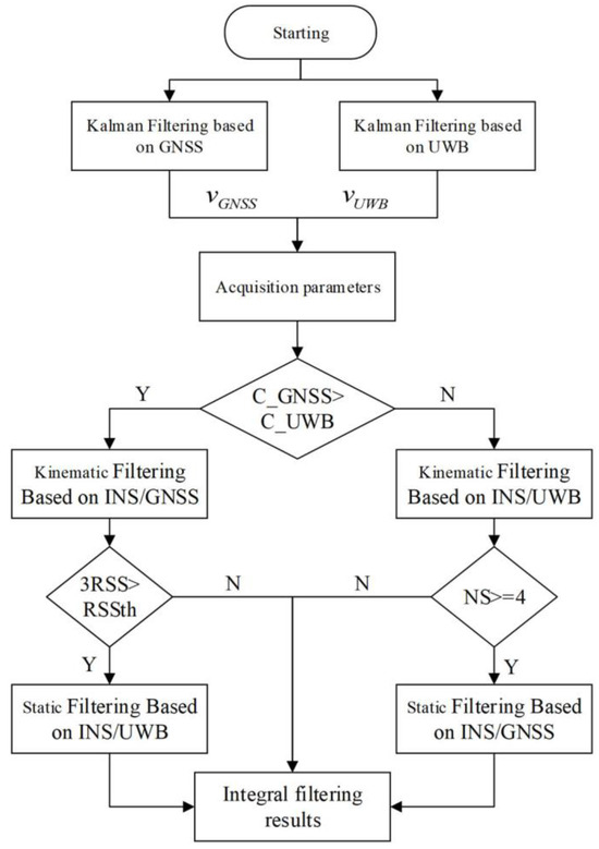
Figure 2.
Structure of INS/GNSS/UWB adaptive robust ESKF kinematic and static filtering based on cost function.
To obtain the positioning residuals of the two positioning systems, GNSS and UWB, in real time, the standard Kalman filtering based on GNSS and UWB was performed first in this algorithm, respectively. After obtaining the RSS, positioning residuals, and positioning stability data of the two navigation systems, the cost function was used to make a judgment. If the cost function of the GNSS was larger than that of UWB, then the kinematic filtering based on INS and GNSS was carried out first. After that, the RSS of UWB at the current moment was judged, and if the RSS of the three base stations for UWB were greater than the threshold, the kinematic filtering results and the covariance of results was passed to the static filtering, and the static filtering based on INS and UWB was carried out. Finally, the static filtered result was output as the overall filtered result. If the three base stations for UWB did not satisfy the conditions, the filtered result of the kinematic filtering was output as the overall filtered result. When the cost function of GNSS was smaller than that of UWB, firstly, the kinematic filtering based on INS and UWB was carried out, and secondly, the number of visible stars of GNSS was judged to be larger than 4. If it was larger than 4, the static filtering based on INS and GNSS was performed and the static filtering result was output, and if it was smaller than 4, the kinematic filtering result was output.
In Figure 2, and are the positioning residuals obtained by standard Kalman filtering enough for GNSS and UWB, respectively, with as an example, and the specific expression for the moment is as follows:
where is the measurement vector at the moment , is the measurement design matrix at the moment , is the state transfer matrix from to , and is the state estimation vector at the moment . C_GNSS and C_UWB are the cost functions of GNSS and UWB, respectively, NS is the number of visible stars of GNSS, and RSSth is the threshold value of RSS signal strength.
4. Simulation Experiment and Result Analysis
4.1. Trajectory Simulation and Parameter Settings
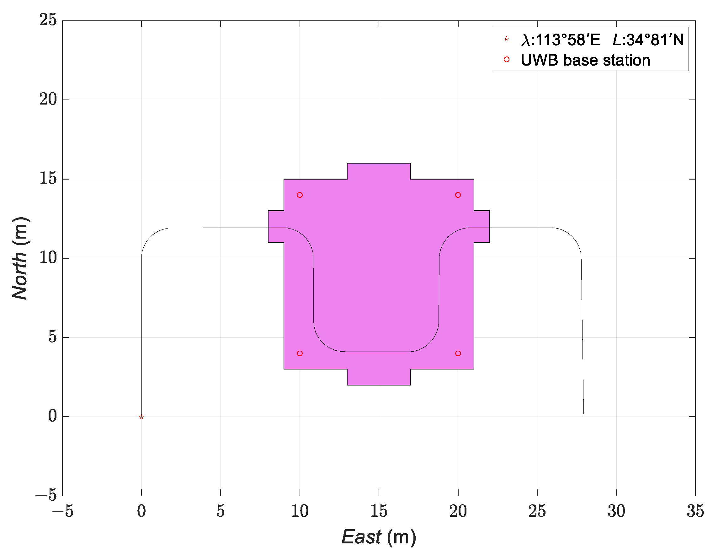
In this paper, the coordinate systems of the three navigation systems are unified into the navigation coordinate system by the quaternion coordinate-transformation method. The chip of the base station for the UWB simulation experiment is DW1000, and time difference of arrival (TDOA) algorithm was used to receive signals emitted by the tags mounted on the carriers and carry out the positioning; the UWB base station deployment is shown in Figure 3, where the red triangles represent the UWB base station. To simulate the positioning effect of the proposed algorithm in indoor and outdoor environments, a brick house was set up as the indoor scene in this experiment, as indicated by the purple area in Figure 3. In this paper, an indoor transition region where the GNSS and UWB signals are in the superposition region was also set up to test the performance of the algorithm proposed in this paper, and the specific region can be seen in Table 2.

Figure 3.
Real trajectory simulation.
Table 2.
Simulation trajectory segment setting table.
To verify the effect of INS/GNSS/UWB adaptive robust ESKF kinematic and static filtering based on the cost function, relevant simulation experiments were conducted in this paper, which set up the real operation trajectory. The initial position was east longitude , north latitude , represented as an asterisk point in Figure 3, the initial attitude (heading angle, traverse roll angle, and pitch angle) were , and the initial velocity were .
According to the above simulation setup, the reference trajectory obtained is shown in Figure 3.
In this paper, we set the systematic errors of the IMU, GNSS, and UWB sensors, and the settings of the carrier sensor parameters are shown in Table 3.
Table 3.
Simulation trajectory segment setting table.
To verify the robustness of the algorithm proposed in this paper under complex environments, the systematic error of UWB was set to be 10 times that of the initial error in the outdoor scene (10 times for example), the velocity systematic error , and the positional systematic error . In the indoor scene, the system error of GNSS was set to be 10 times that of the initial error, the velocity system error , and the position system error . In the indoor–outdoor transition phase, the system errors of both GNSS and UWB were 5 times that of the initial error, and the GNSS and UWB positioning systems were normal at other times.
To compare the relevant performance of the algorithm proposed in this paper, three filtering solution schemes were set up. In the process of setting up the filtering schemes, the ESKF-based federated filter was used in Scheme 1 for the experiments. Scheme 2 shows the kinematic and static filtering using ESKF based on INS/GNSS/UWB. Scheme 3 shows the algorithm proposed in this paper.
4.2. Simulation Results and Analysis
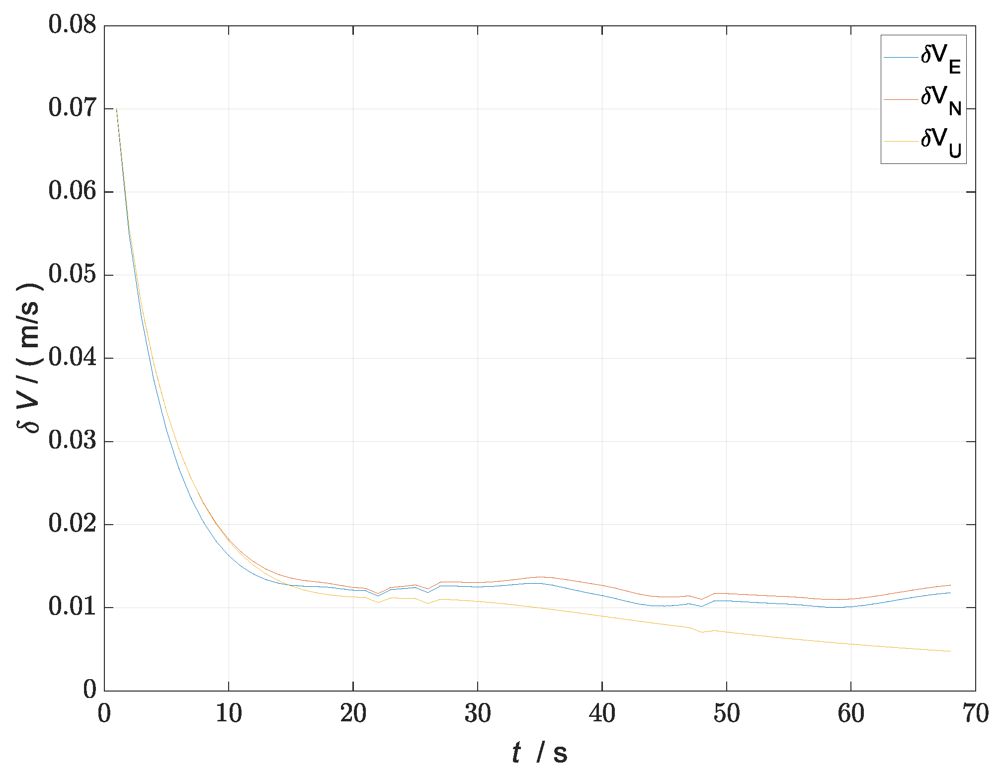
We set the velocity measurement noise of both INS/GNSS sub-filter and INS/UWB sub-filter to and set the position measurement noise to for the related simulation. The simulation results of filtering velocity error and position error are shown in Figure 4 and Figure 5.
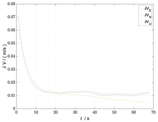
Figure 4.
Diagram of velocity error.
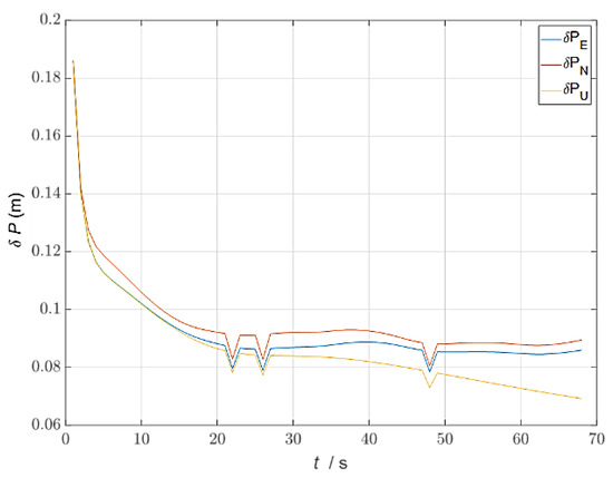
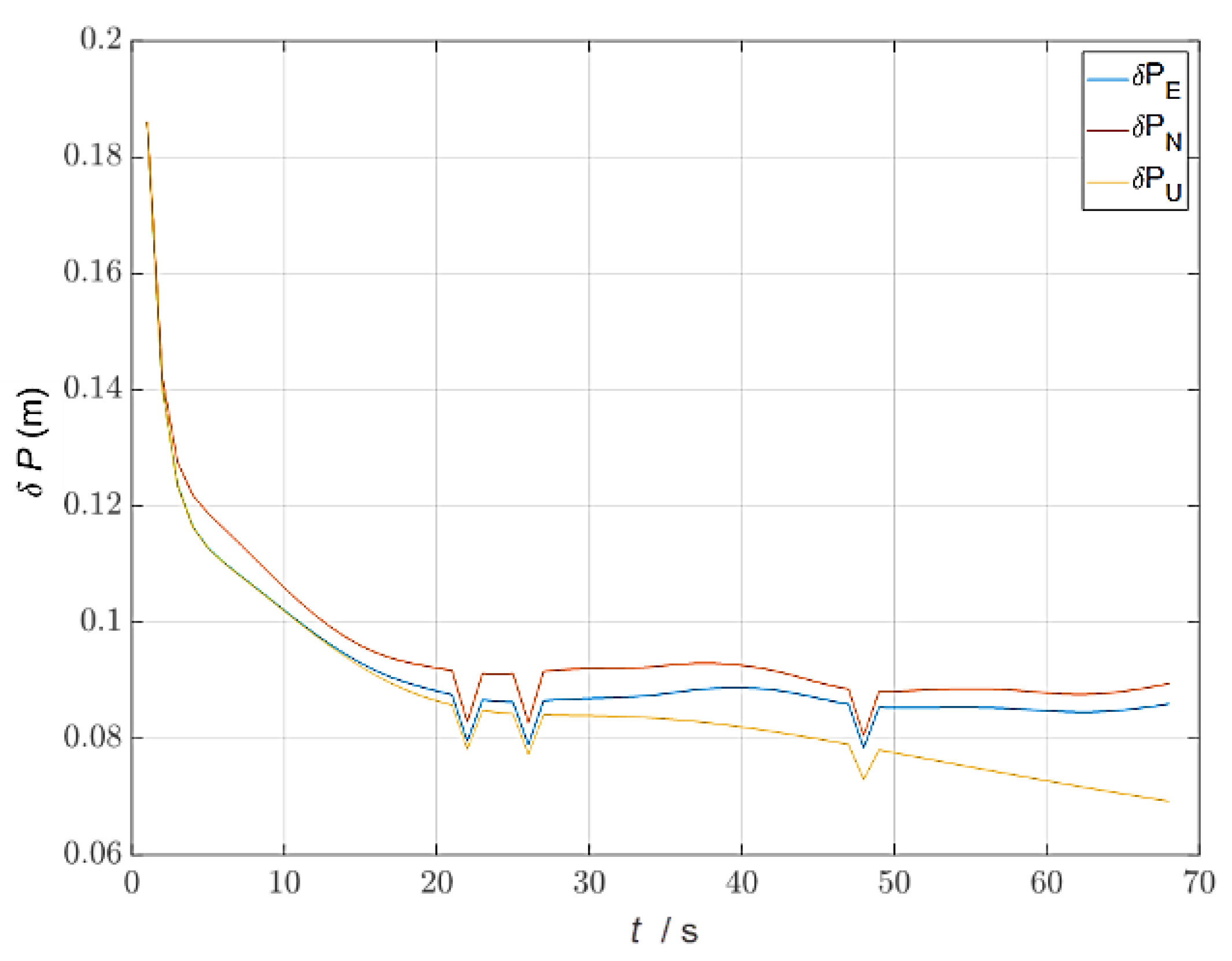
Figure 5.
Diagram of position error.
According to Figure 4 and Figure 5, it is shown that the filtering velocity error converges around 20 s and converges to 0.01 m/s, the position error converges around 20 s and finally converges to 0.09 m, and the position error jitters at 23 s, 26 s, and 49 s. The specific reason for the jitter is that the filtering structure of the carriers in the indoor/outdoor transition region is altered according to the cost function, but through the change in the filtering by the above analysis, it can be proved that the position error and velocity error of the overall filter in the algorithm proposed in this paper have convergence.
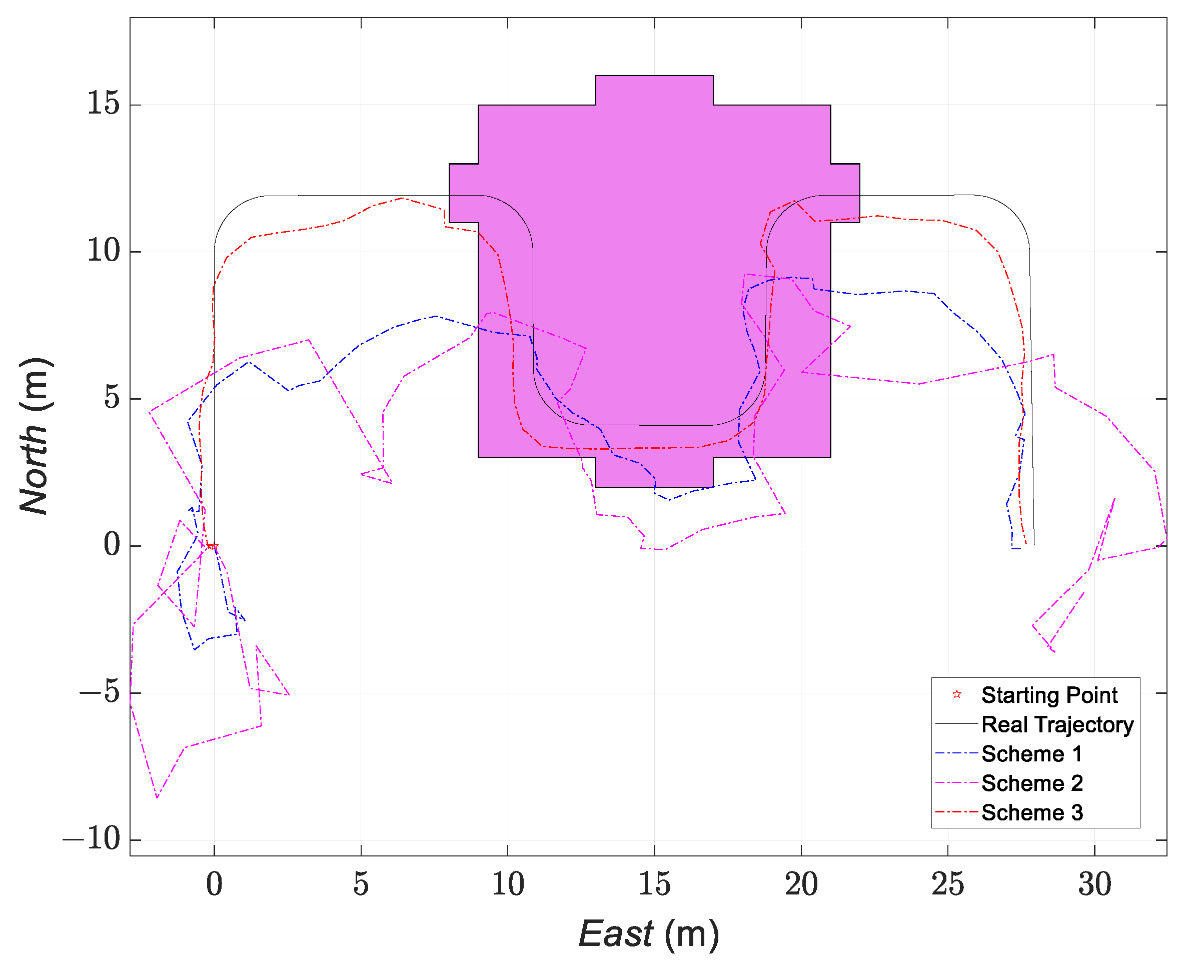
After simulating the comparison experiments, the results of trajectory comparison for Scheme 1, Scheme 2, and Scheme 3 are shown in Figure 6.
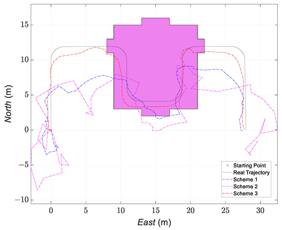
Figure 6.
Comparison of the trajectories of the three schemes.
In Figure 6, the star-shaped point is the origin point of UGV motion, and the black trajectory is the real simulation trajectory. According to Figure 6, it can be seen that the simulation trajectory of the proposed algorithm in this paper is much closer to the real trajectory compared to the simulation trajectories of the other two schemes.
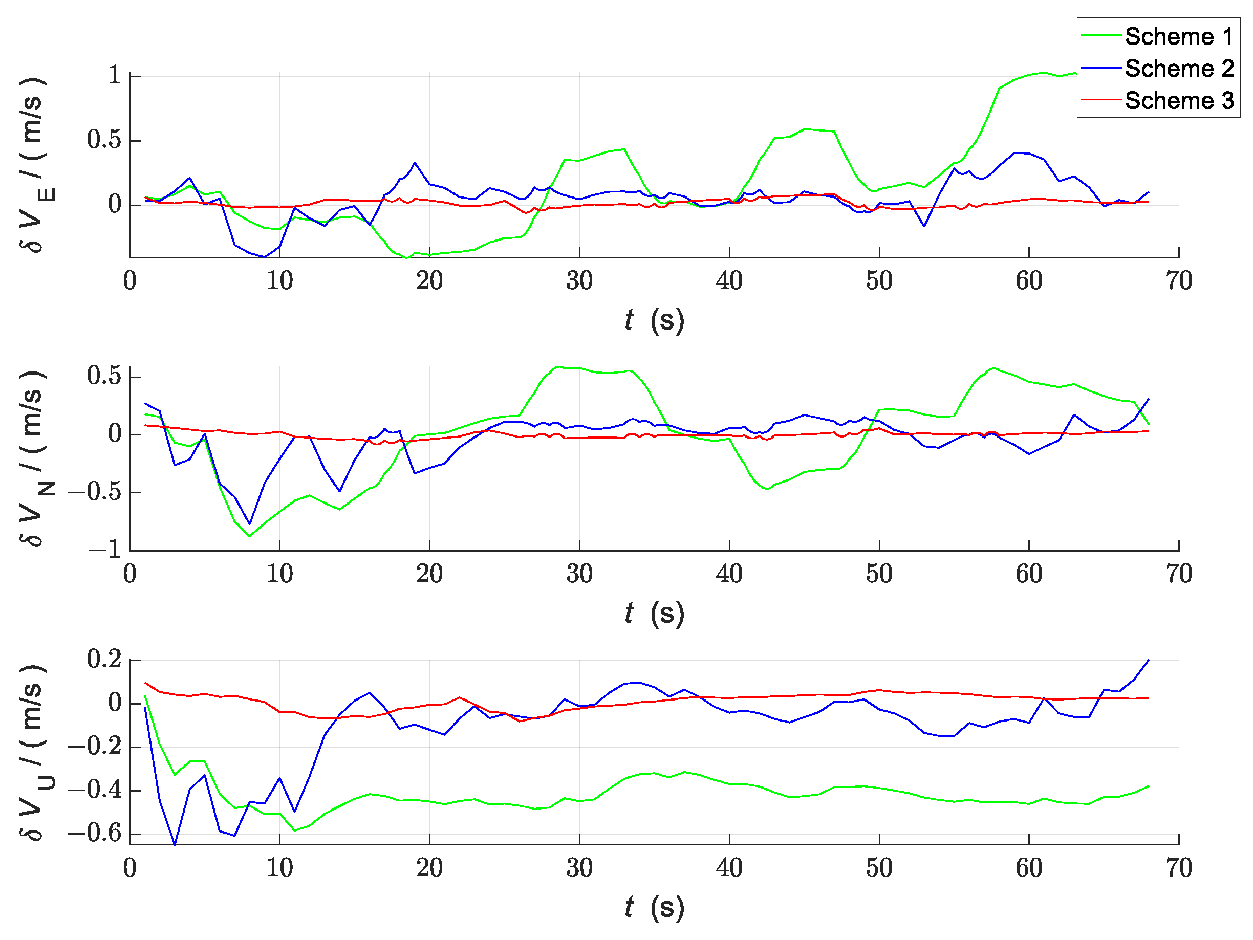
The speed error comparison and position error comparison of the three simulation schemes are shown in Figure 7 and Figure 8, respectively. In Figure 7 and Figure 8, the green solid line represents the velocity and position error versus time curves in Scheme 1, the blue color represents the velocity and position error versus time curves in Scheme 2, and the red color represents the velocity and position error versus time curves in the INS/GNSS/UWB adaptive robust ESKF kinetic and static filtering based on the cost function proposed in this paper.
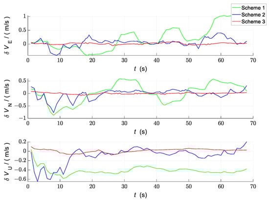
Figure 7.
Comparison of velocity errors between the three schemes.
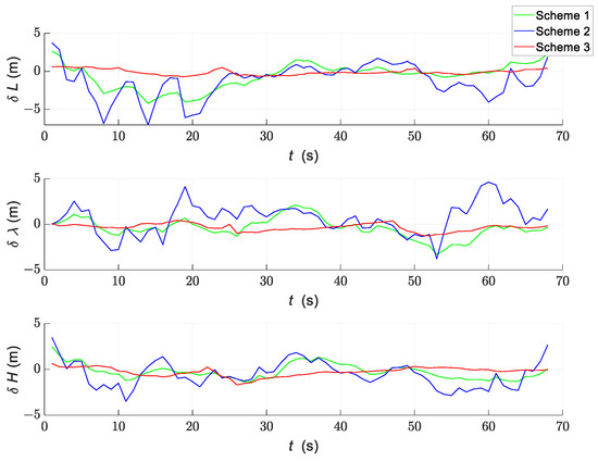
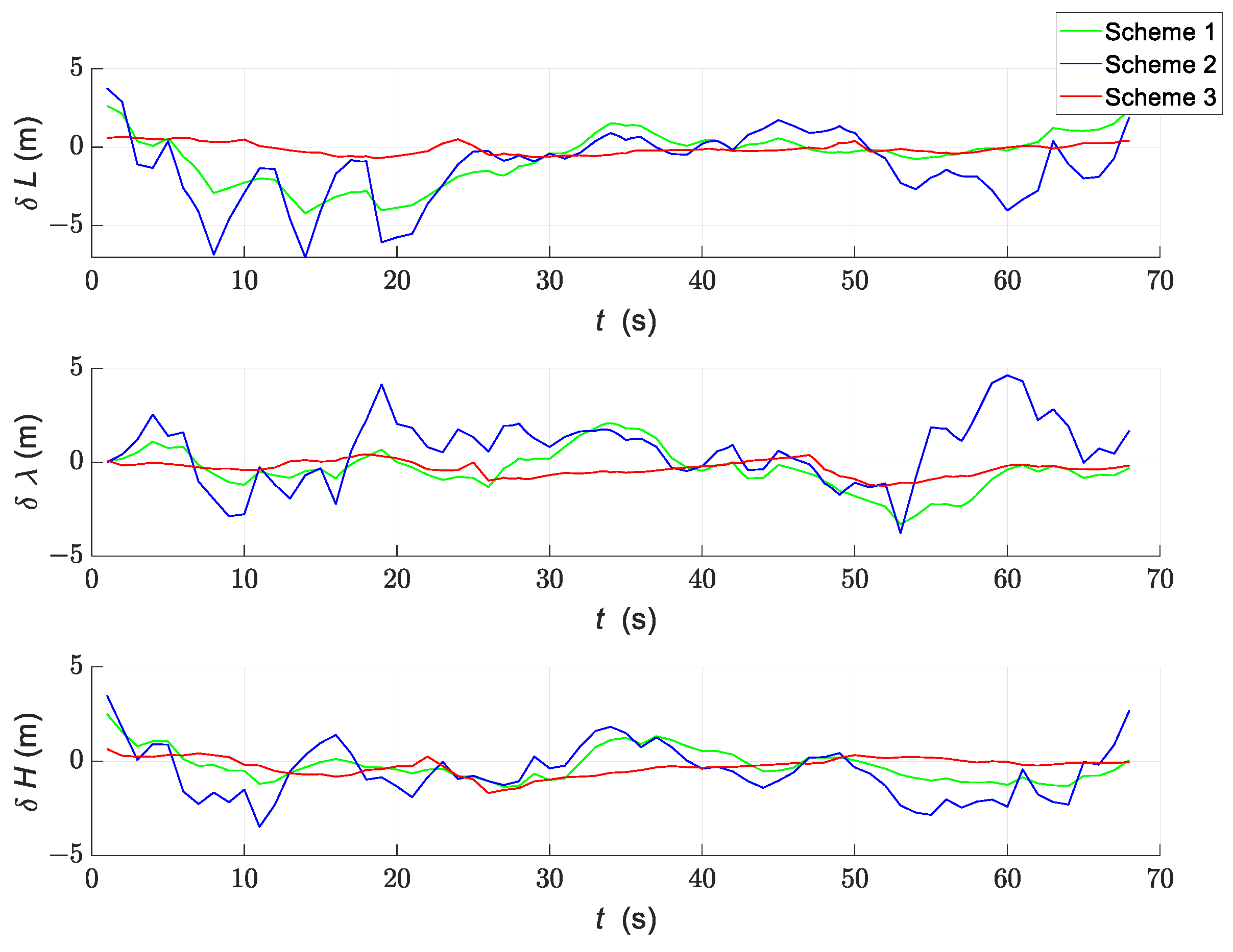
Figure 8.
Comparison of position errors between the three schemes.
According to Figure 7 and Figure 8, it can be seen that regarding the proposed algorithm in this paper, compared with the other two schemes, the velocity errors in the eastward, northward, and skyward directions are greatly reduced, and the average value is around 0.4 m/s, while the absolute values of the position errors in the longitude (eastward), latitude (northward), and ellipsoidal altitude (skyward) are smaller than those of Scheme 1 and Scheme 2, and the change curves of the errors are smoother, which is mainly due to the the proposed algorithm in this paper. The main reason is that the algorithm proposed in this paper autonomously shields the contaminated GNSS and UWB in the filtering according to the cost function, so that the overall filtering performance is improved. The comparison of the root mean square error of attitude, position, and velocity of the three navigation modes and the comparison of the average absolute value error are shown in Table 4 and Table 5.
Table 4.
Comparison of the root mean square error (RMSE) of the three schemes.
Table 5.
Comparison of the mean absolute error (MAE) of the three schemes.
According to Table 4, the overall speed rms error of the proposed algorithm in this paper is reduced by 92.09% compared to Scheme 1 and 61.16% compared to Scheme 2; the overall position rms error is reduced by 81.41% compared to Scheme 1 and 74.44% compared to Scheme 2. According to Table 5, it can be seen that the overall speed mean absolute value error in the algorithm proposed in this paper is reduced by 92.31% and that the overall position mean absolute value error is reduced by 60.01% compared to Scheme 1; the overall speed mean absolute value error is reduced by 77.64% and the overall position mean absolute value error is reduced by 74.16% compared to Scheme 2.
5. Conclusions
In this paper, a fusion navigation algorithm of INS/GNSS/UWB adaptive robust ESKF kinematic and static filtering based on cost function is proposed, which constitutes a cost function by selecting RSS, positioning residual, and positioning stability as parameters, and normalizing and assigning weights to different parameters according to the parameter judgment matrix. On this basis, taking the seamless switching scene between indoor and outdoor as an example, the cost function is introduced into the kinematic and static filtering so that the overall filtering carries out autonomous judgment on the subsystems and adaptively changes the filtering structure according to the judgment results, thus improving the overall positioning accuracy of the filtering. Through simulation experiments and control experiments, the positioning accuracy based on the algorithm proposed in this paper is improved by 75.9% and 74.44% compared with the INS/GNSS/UWB-based federated filter and the INS/GNSS/UWB-based ESKF kinematic and static filters that do not use the cost function, and the overall filtering is not dispersed because of the structure switch. Therefore, the algorithm proposed in this paper can effectively reduce the error generated by the fused autonomous navigation due to the contamination of the subsystem and can effectively improve the dependable decision-making ability and robustness of the fused autonomous navigation system, which can be effectively applied to the seamless switching scene between indoor and outdoor.
Author Contributions
Z.R., S.L., J.L., J.L., J.D. and Y.L. conceived and designed the study; Z.R. designed and performed the simulation experiments; S.L. and J.L. optimized the experiments; Z.R. wrote the paper; S.L., J.L., J.D. and Y.L. reviewed and edited the manuscript. All authors have read and agreed to the published version of the manuscript.
Funding
The research was supported by the National Natural Science Foundation of China (NO. 60171009) and the project Research on key technology of intelligent air-ground unmanned systems for au-tonomous co-operation and high dynamic tracking and landing (NO. 242102210028).
Institutional Review Board Statement
Not applicable.
Informed Consent Statement
Not applicable.
Data Availability Statement
Data sharing is not applicable due to privacy.
Conflicts of Interest
The authors declare no conflicts of interest.
References
- Wei, W. Research on Basic Characteristics of Multi-source Autonomous Navigation System. J. Astronaut. 2023, 44, 519–529. [Google Scholar]
- Wang, W.; Wu, Z.; Meng, F.; Xu, X.; Wu, S. Research on Dependability of Multi-source Autonomous Navigation System. Navig. Control 2023, 22, 1–9. [Google Scholar]
- Shen, C.; Wang, C.; Zhang, K.; Wang, X.; Liu, J. A time difference of arrival/angle of arrival fusion algorithm with steepest descent algorithm for indoor non-line-of-sight locationing. Int. J. Distrib. Sens. Netw. 2019, 15, 1550147719860354. [Google Scholar] [CrossRef]
- García, E.; Poudereux, P.; Hernández, Á.; Ureña, J.; Gualda, D. A Robust UWB Indoor Positioning System for Highly Complex Environments. In Proceedings of the IEEE International Conference on Industrial Technology, ICIT 2015, Seville, Spain, 17–19 March 2015; pp. 3386–3391. [Google Scholar]
- Kuang, J.; Niu, X.; Chen, X. Robust Pedestrian Dead Reckoning Based on MEMS-IMU for Smartphones. Sensors 2018, 18, 1391. [Google Scholar] [CrossRef] [PubMed]
- René, H. Seamless Indoor/Outdoor Positioning Handover for Location-Based Services in Streamspin. In Proceedings of the Tenth International Conference on Mobile Data Management: Systems, Services and Middleware, Taipei, Taiwan, 18–20 May 2009; pp. 267–272. [Google Scholar]
- Yang, F.; Aoshuang, D. A Solution of Ubiquitous Location Based on GPS and Wi-Fi ULGW. In Proceedings of the Ninth International Conference on Hybrid Intelligent Systems, Shenyang, China, 12–14 August 2009; pp. 260–263. [Google Scholar] [CrossRef]
- Deng, Z.; Zhu, Y.; Wang, H. Cost Function of Features Based Mode Switching Algorithm for Indoor Positioning. In Proceedings of the 5th International Conference on Wireless Communications, Networking and Mobile Computing, Beijing, China, 24–26 September 2009; pp. 1–4. [Google Scholar]
- Wu, M. Research of Handover Algorithm Based on Fuzzy Logic Control For Seamless Navigation System; Harbin Institute of Technology: Harbin., China, 2012. [Google Scholar]
- Hassen, W.; Najjar, F. A Positioning Technology Switch Algorithm for Ubiquitous Pedestrian Navigation Systems. In Proceedings of the IEEE 13th International Conference on Embedded and Ubiquitous Computing, Porto, Portugal, 21–23 October 2015; pp. 124–131. [Google Scholar] [CrossRef]
- Ren, Z.; Liu, S.; Dai, J.; Lv, Y.; Fan, Y. Research on Kinematic and Static Filtering of the ESKF Based on INS/GNSS/UWB. Sensors 2023, 23, 4735. [Google Scholar] [CrossRef] [PubMed]
- Yorozu, T.; Hirano, M.; Oka, K.; Tagawa, Y. Electron Spectroscopy Studies on Magneto-Optical Media and Plastic Substrate Interface. IEEE Transl. J. Magn. Jpn. 1987, 2, 740–741. [Google Scholar] [CrossRef]
- Zhenyao, L. Research on Technology of Seamless Positioning Based-on UWB/GNSS/MIMU; Information Engineering University: Henan, China, 2017. [Google Scholar]
Disclaimer/Publisher’s Note: The statements, opinions and data contained in all publications are solely those of the individual author(s) and contributor(s) and not of MDPI and/or the editor(s). MDPI and/or the editor(s) disclaim responsibility for any injury to people or property resulting from any ideas, methods, instructions or products referred to in the content. |
© 2024 by the authors. Licensee MDPI, Basel, Switzerland. This article is an open access article distributed under the terms and conditions of the Creative Commons Attribution (CC BY) license (https://creativecommons.org/licenses/by/4.0/).