Automated Damage and Defect Detection with Low-Cost X-ray Radiography Using Data-Driven Predictor Models and Data Augmentation by X-ray Simulation ^†

Abstract

The detection of hidden defects in materials using X-ray images is still a challenge. Often, a lot of defects are not directly visible in visual inspection. In this work, a data-driven feature marking model is introduced to perform semantic pixel annotation. Input data are delivered by a standard industrial X-ray instrument and a low-cost self-constructed portable X-ray instrument, which is introduced in detail in this work, too. The technical details of the X-ray instrument are relevant since the quality of the feature detector is compared with respect to noise, contrast, and signal quality. Finally, a simulation of X-ray images is used to provide a ground truth data set for the training of the feature detector. It is shown that this approach is suitable for detecting hidden pores in high-pressure die-casted aluminum plates.

1. Introduction

It is still difficult to identify and detect hidden faults or impurities in multi-layered composites like fiber-metal laminates (FML), as well as in homogeneous materials, e.g., high-pressure die-casted aluminum materials, even using advanced X-ray Computer Tomography (CT). For example, an impact damage can be nearly invisible using a frontal X-ray projection, although the deformation can be seen and detected manually by hand perception. Hidden pores in materials can be detected and analyzed by 3D CT volume rendering, but they are hard to identify in single projection images (radiography). Things become worse if a portable low-cost X-ray radiography or semi-tomography machine is used (called a LowQ measuring device), as introduced and described in this work.

It is desirable to detect or mark defects, damages, or impurities using an automated feature marking system directly in the measure images. The impact of image quality can be relevant to the feature detection quality, regardless of the complexity of the model behind [1]. Often, complex neural networks (deep learning models) are used [2]. In this work, a simple pixel classifier is used. Semantic pixel detectors are simple mathematical models that can be used to mark Regions of Interest (ROIs) in an image relating to a specific semantic class. After the image preprocessing and filtering stages, damage and material faults are identified by a pixel anomaly detector, basically an advanced Convolutional Neural Network (CNN) and region proposal R-CNN models. Training pixel classifiers can require the use of only a few images because each pixel region is a sample instance. R-CNN models require an extended sample data base which cannot be acquired only by physical measurements. The training and test data set will always be limited by a limited number of specimens, e.g., with impact damages, and a limited variance in material and damage parameters (e.g., location). For this reason, the data set is extended by synthetic data augmentation using X-ray simulation. In contrast to other wave measurement principles like Guided Ultrasonic Waves (GUWs), X-ray images can be simulated with high accuracy (compared with physically measured images). We are using the gVirtualXray software library [3,4] and performing X-ray image simulation by using GPU processing only and ray tracing. gVirtualXray is proven in terms of its suitability to produce accurate images as long as the diffraction and reflection of X-rays are neglected. In addition, a novel few projection hidden-damage detection methodology is introduced that can be used in-field with a portable X-ray machine as described above. Preliminary results show a high defect detection rate for a wide range of materials.

An X-ray measuring system (see Figure 1, left) consists of an X-ray source (commonly a cone beam with a specific focal size diameter fsd) and an X-ray detector. The X-ray source uses either a cold emission or hot emission (Coolidge) X-ray tube. In cold emission, the electrical field extracts and accelerates electrons from the cathode to the anode; in hot emission, there is a heated free electron source, and the electrical field only accelerates the electron to a target anode material. Cold emission tubes lack independent tube current control (dependent on the tube voltage).

The X-ray detector can be a direct or indirect conversion system. In a direct conversion system, the X-ray photons will generate electrons (photo effect) directly in the solid-state device; in an indirect conversion system, a conversion material (scintillator) is required to convert X-ray photons into visible light photons, which are finally converted to electrons in a solid-state detector.

In addition to the X-ray conversion mode, there are direct coupled detectors and imaging systems that map the X-ray converted image from a scintillator onto a solid-state detector. Direct coupled systems require an optical coupling material, commonly a fiber optic plate (FOP) posing high geometric accuracy and low distortion. An indirect imaging system with a lens-based imaging system can introduce optical distortion and yield reduced geometric accuracy, but these types of systems have the advantage of being inexpensive [5].

Solid-state detectors are typically Coupled Charge Devices (CCDs) or CMOS pixel detectors. Despite the fact that when used in an indirect conversion system, they are sensitive to visible light, they are still sensitive to incident X-ray radiation producing shot or popcorn noise.

The X-ray equipment consists of a low-cost X-ray source for dental diagnostics and an X-ray detector consisting of a conventional medical X-ray converter and amplifier foil (Fine 100) backside imaged by a commercially available CMOS monochrome image sensor (back-illuminated Sony IMX290 2 M pixel sensor, described later) and a simple two-lens optics. The optical distortion introduced by the optics increases with increasing distance from the center of the image (“barrel distortion”) and must be corrected, at least for CT 3D volume reconstruction.

The measured X-ray images pose increased gaussiand- and non-gaussian distributed noise (compared with high-quality flat panel detectors) and more important randomly located “popcorn” shot noise by avalanche effects in pixels and pixel clusters (islands) due to X-ray radiation exposure (back-illuminated sensors are very sensitive to this noise). The gaussian noise can be reduced by averaging; the shot noise is removed by using multiple images recorded in series and an automated pixel replacement algorithm. The shot noise is a seed threshold phenomenon, i.e., the location and number of white pixels changes from image to image, therefore allowing for the replacement of white pixels in one image from unaltered pixels from another image.

Basically, we can classify X-ray measuring devices and systems into three classes with respect to non-destructive testing (NDT) in engineering, especially for metals and composite materials:

• HighQ: Micro CT devices with micro focus tubes with optional optical magnification (focal spot diameter below 50 μm), effective resolution below 100 µm;
• MidQ: Industrial systems (standard focal spot diameter above 100 μm, typically 0.8 mm), effective resolution above 100 µm;
• LowQ: Low-cost system (standard focal spot diameter above 100 μm, typically 0.8 mm), effective resolution above 30 µm.

The classification quality relies on resolution, contrast, and noise. In the following section, we only distinguish between a low-cost and self-constructed LowQ and an industrial MidQ instrument as a reference with standard focal spot diameters of about 0.8 mm. The low-cost X-ray measuring instrument (<EUR 1000) should be an alternative for laboratory and industrial devices that are much more expensive (>EUR 100,000). The technical and construction details are important for comparing the device classes.

In addition to the description and evaluation of the LowQ X-ray measuring system used for NDT applications (Section 2), we investigate X-ray image simulation, discussed in Section 3, finally used for the training of ML defect detection models (Section 4). The overal framework addressed in this work is shown in Figure 1.

2. X-ray Radiography and CT Systems

Two experimental setups, delivering input data for the training and testing of the automated damage feature marking model, are described in this work:

• MidQ: A laboratory radiography and CT system (Fraunhofer IFAM, Yxlon Y.MU2000-D, Hamamatsu detector), electron beam focus spot diameter—0.75 mm (Wolfram anode material), anode voltage—50–120 kV, tube current up to 10 mA, direct imaging solid-state detector 1000 × 1000 pixels, detector pixel size—200 μm.
• LowQ: A self-constructed, mobile, low-cost radiography and CT system, electron beam focus spot diameter 0.8 mm (Wolfram anode material), anode voltage 30–70 kV, tube current up to 1 mA, indirect imaged monochrome and back-illuminated CMOS camera sensor (1920 × 1080 pixels), detector pixel size—3 μm, image-scaled virtual detector pixel size—40 μm, X-ray scintillator screen (Ortho Fine 100 foil).

2.1. Low-Cost X-ray Device

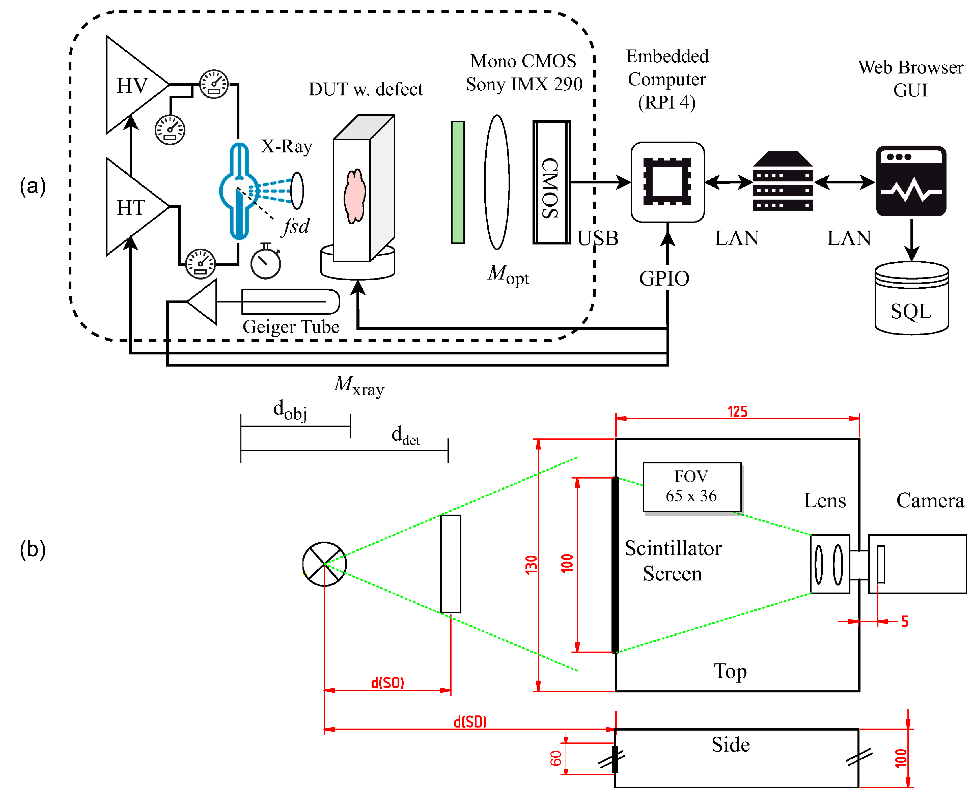
The first device is only a reference system used to derive material and structure models and to compare with the low-cost system introduced in this work. The architecture and the main components of the proposed low-cost LowQ X-ray measuring device are shown in Figure 2. A low-cost commercial wolfram X-ray tube with a focal spot diameter of 0.8 mm and a typical anode voltage range of 30–80 kV is used. The imaging system consists of a widely used X-ray intensifier screen (Ortho Fine 100) and a commercial CMOS camera with double-lens optics. The entire X-ray measuring device is controlled by an embedded computer (Raspberry Pi 4). The camera and the device controls can be accessed remotely via a Web browser.

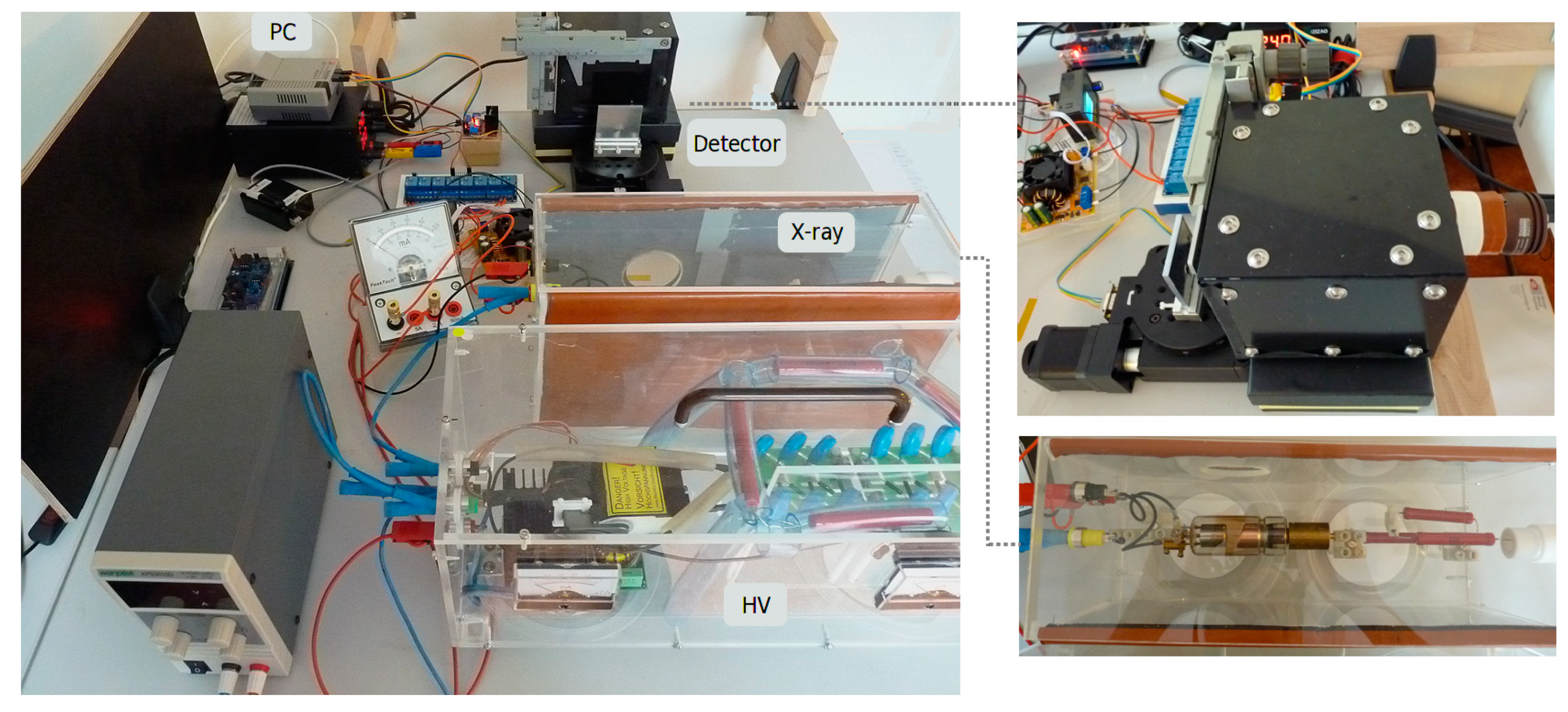
The X-ray tube is a KL 27-0.8-70 based on a classical Coolidge principle (hot emission tube). The focal spot diameter is about 0.8 mm, with an opening angle of 19° (i.e., 70 mm spot diameter at 200 mm distance). The X-ray beam current can be controlled by the heater independently from the X-ray anode voltage (maximal tube current is 10 mA). Nearly most of the electrical input power is converted into heat in the tube anode. Even low tube currents of about 1 mA produce a heat power of more than 50 W, raising the temperature of the anode far beyond 100 °C (measured using a thermal camera). The heat must be propagated outside the tube; here, it is propagated by an attached massive Cooper cylinder (see the right side of the tube in Figure 3 for a detailed view of the X-ray source) and a ventilator. With this cooling, the anode temperature can be kept below 40 °C for operating times below one minute.

The camera consists of a commercial monochrome CMOS back-illuminated image sensor (Sony IMX 290, Omegon Kamera Guide 2000 M Mono), providing 1920 × 1080 pixels with 3 μm × 3 μm pixel size. The CMOS sensor supports high exposure times (5 s and longer) by posing low-noise output. The optical imaging system consists of a zoomable double-lens system that maps the backside of the scintillator screen on the image sensor. With the given distance of 125 mm (see Figure 2b) between screen and image sensor, the effective Field of View (FOV) is about 65 × 36 mm (effective image size is 30 μm).

The X-ray source unit, the X-ray detector unit, and the optional rotation stage are controlled by an embedded computer (Raspberry Pi 4), which is connected to a LAN. The instrument can be accessed via a Web browser. There is one main application program running on the embedded computer. The program controls the camera (using a vendor SDK, ToupTek photonics, http://www.touptek.com/) and captures images via USB, the X-ray unit, and a rotation stage stepper motor via a GPIO port. A Geiger counter is used to monitor the X-ray intensity. The remote access is provided via a HTTP service, providing the HTML control page, too (embedded in the software).

2.2. Electronics

An electronic schematic of the X-ray source is shown in Figure 4. The circuit consists of a high-voltage generator, an electron heater constant current supply, and relay switches connected to the embedded computer. The high-voltage generator uses a classical discrete zero voltage switching (ZVS) driver circuit to drive a high-voltage transformer. The input voltage of the ZVS determines the output voltage of transformer T1 (about 40 kHz; input range: 5–12 V; output voltage: 5–12 kV). The output voltage of the high-voltage transformer is multiplied by a six-stage Villard cascade. The HV supply delivers up to 70 kV and 1 mA current (70 W). Neither the voltage nor the tube current is regulated by a feed-back loop, in contrast to industrial devices.

2.3. Detector

The resolution of an X-ray imaging system is mainly limited by two parameters:

• Detector pixel size d_p multiplied by the optical image magnification, i.e., d_pM_opt;
• The X-ray magnification M_xray.

The X-ray magnification is given by the following:

$$\begin{array}{l}{M}_{xray}=\frac{d_{\det ,src}}{d_{obj,src}}\\ a=\left(M_{xray}-1\right)f_b\end{array}$$

(1)

with f_b as the focal spot diameter (FSD), resulting in an imaging focus limit of about a (aperture limit) [6].

The exposure time t_x defines the noise level and the source-to-noise ratio achievable with the given X-ray power P_x. The industrial reference Mid-Q system has a pixel area size of about 40 kμm², whereas the LowQ detector has a pixel area of only 9 μm²! The direct imaging MidQ system tightly couples the scintillator to the detector pixels via a FOP, whereas the indirect imaging system poses optical losses in lenses and coupling components. The MidQ system typically requires exposure times in the order of 100 ms (with P_x = 200 W), whereas the LowQ device requires at least 5000 ms (with P_x = 50 W).

The camera deployed in the LoWQ device is a USB 2.0 Omegon Guide 2000 M Mono with a back-illuminated monochrome Sony IMX290 sensor. The optical imaging system consists of a CS-Mount double-lens system with 2.8–12 mm focal length and f/1.4 aperture. The IMX290 image sensor uses an integrated 12 Bits ADC (directly accessible by a camera raw format) for image digitalization, while an external 16 Bits ADC is used in the industrial MidQ detector.

The scintillator used in the detector has a normalized conversion factor of 100, providing sufficient amplification and high resolution. The scintillator consists of phosphor materials based upon a mix of rare earths with a high luminous intensity and low graininess. The screen emission matches ideally with the spectral sensitivity of the image sensor, as shown in Figure 5 (relative sensitivity of 0.95 at main emission peak). A limiting resolution up to 10 Line Pairs (LP)/mm with 10% contrast can be achieved. The contrast of the entire low-cost X-ray detector is about 70% at 2 LP/mm and about 25% at 8 LP/mm.

2.4. Noise

The CMOS image sensor is sensitive to X-ray radiation, not too much to warrant the use of the image sensor directly, but with respect to popcorn and shot noise. Popcorn noise is a random seed phenomena; i.e., in some pixels, there is an electron wall breakthrough, leading to saturated (white) pixels. Fortunately, after the pixels are cleared (before the sampling of the next image), the saturation is eliminated, and two succeeding images will commonly not pose the same flooded pixels.

Commonly, the image device is not directly exposed to the X-ray beam. Instead, a mirror under an angle of 45° is used, and the camera is placed with a 90° angle with respect to the X-ray beam axis (see [5]). We tried the same approach, but we observed the following:

• An expected reduction in light intensity (mirror reflectivity < 1) and more geometric distortions.
• There is still shot noise (albeit strongly reduced but not totally vanished).

The second observation is a result of the mirror construction. The mirror was a conventional industrial aluminum mirror mounted on an aluminum carrier under the same angle as the mirror. This combination still scatters some X-rays.

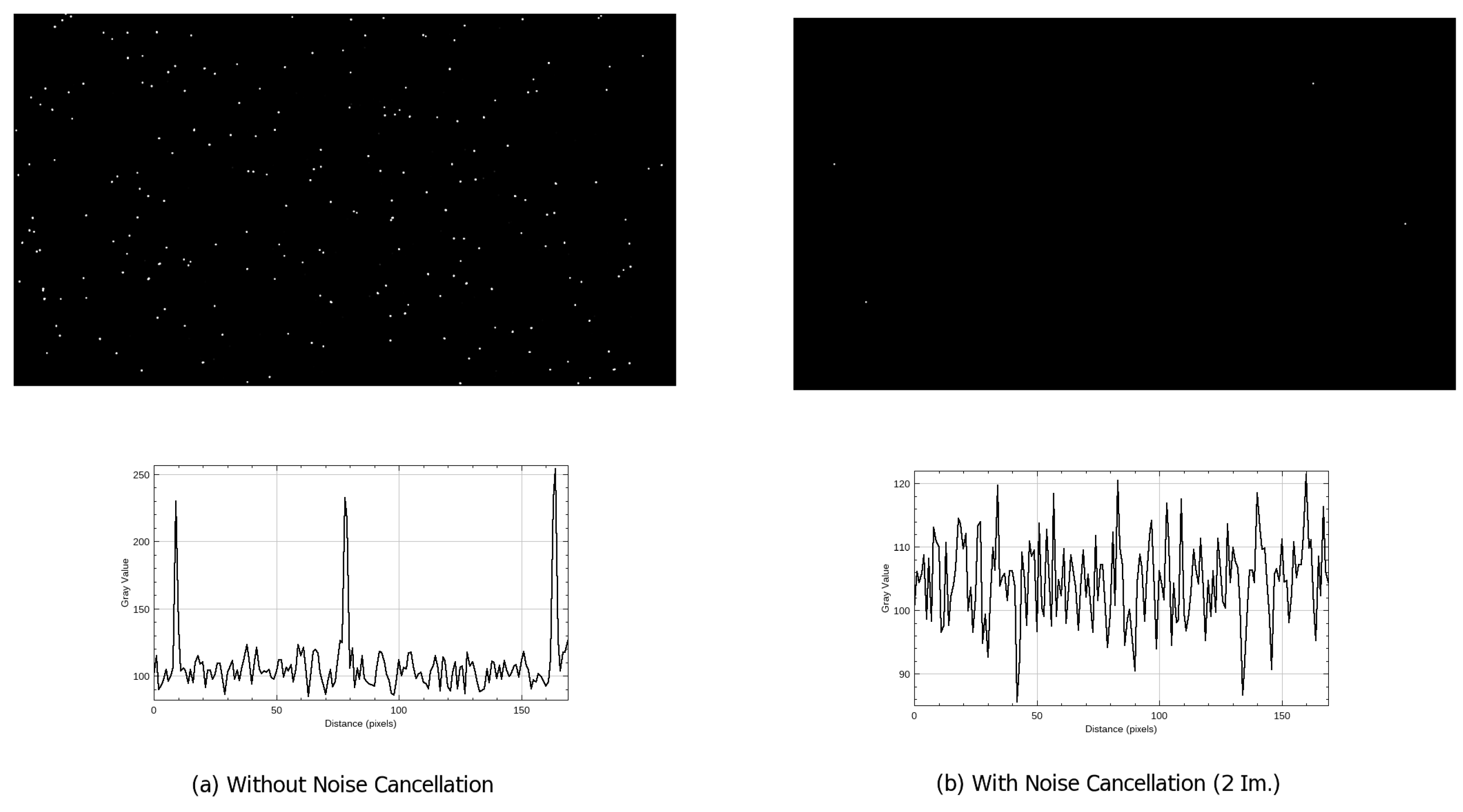
Therefore, we placed the camera in the X-ray beam again and used a simple multi-image noise compensation method. This removes shot noise and reduces non-gaussian X-ray and gaussian (electronics) noise, as shown in Alg. 1. Examples and results are shown in Figure 6. Choosing the γ threshold is crucial because not all shot noise pixels reach the maximum camera intensity, and some will only be reduced by averaging if they are below the chosen threshold, as shown in Algorithm 1.

Algorithm 1: Shot (popcorn) noise removal and image averaging. γ is a noise threshold with respect to the image pixel value range (commonly 0.9max), and Σ is a set of images. The result of the averaged and noise-corrected image is σ0.

σ0 := Σ[1]

∀ (x,y) ∈ coord(σ0) do

if σ0[x,y] > γ then

∀ σ ∈ {Σ/σ0} do

if σ[x,y] < γ then

σ0[x,y] := σ[x,y]

break

endif

done

endif

∀ σ ∈ {Σ/σ0} do

if σ[x,y] < γ then

σ0[x,y] := σ0[x,y] + σ[x,y]

else

σ0[x,y] := σ0[x,y] + σ0[x,y]

endif

done

σ0[x,y] := σ0[x,y]/|Σ|

done

In addition to the shot noise, there is gaussian electronics and detector noise (not correlated among pixels) and non-gaussian X-ray radiation and source noise, which can pose spatial correlation. In Section 5 and Figure 10, the gaussian noise of the images sampled by the LowQ and MidQ instruments are compared. The industrial MidQ device (including the X-ray source) has an average noise level of SNR = avg(x)/σ = 280 (the 2σ noise interval is about 0.7%), whereas the LowQ device has an SNR = 95 (the 2σ noise interval is about 2%).

3. Simulation

As is common in engineering applications, the data variance of the experiments and specimens is limited. On one hand, specimens with impact damage pose a wide range of different micro and macro damages (e.g., delaminations, cracks, kissing bond defects, and many more). Therefore, the measurement (X-ray image) of one specimen delivers only a few features, and the number of specimens is limited, too. High-pressure die-casted aluminum specimens, on the other hand, contain a high number of gas pores (herein named defects), and the number of specimens can be high. Even if the feature and data variance is sufficient, there is no ground truth in the data, which is specifically required for the accurate labeling of training data for supervised Machine Learning (ML). For this reason, in this work, X-ray images are computed (simulated) numerically from synthetic specimens based on a CAD model and Monte Carlo simulation techniques, as shown in Figure 7. The model is composed of Constructive Solid Geometry operations creating solid materials or defects (pores) by union or difference operations. The OpenSCAD software [9] was used to convert the CSG model into a triangular mesh grid model (STL). This mesh model was finally processed by our own X-ray simulation software [10] based on the gvxr/gVirtualXray C++ software library [3] for the computation of X-ray images.

The Monte Carlo simulation of the synthetic pores was based on a simple geometric ellipsoid model with a base parameter set derived from real pore analysis using CT reconstruction and projections measured using the MidQ device.

4. Feature Detection Using a Semantic Pixel Classifier

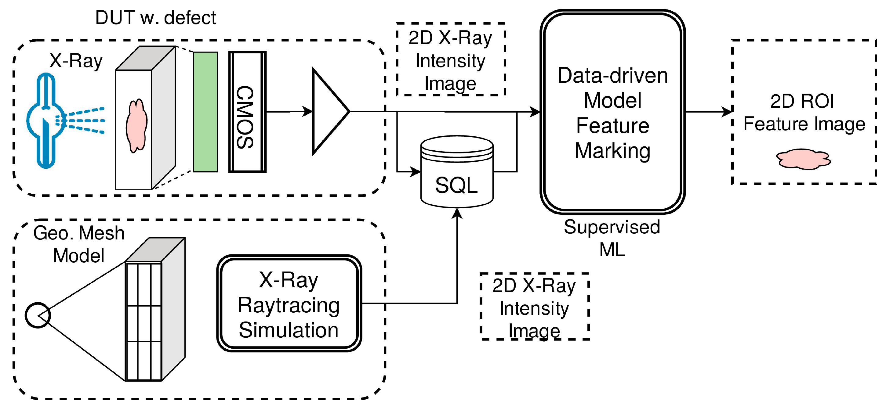
The main objective of this work is to use an automated feature detector and apply it to single projection X-ray images delivered by a Low-Q (low-cost) X-ray instrument to detect hidden defects in materials (which, in the context of this study, are pores in high-pressure die-casted aluminum plates).

The input is an X-ray image; the output is a feature map image that marks pores and provides the geometric parameters and position, as shown in Figure 8. A pixel classifier is commonly implemented with a Convolutional Neural Network (CNN), mostly with only one or two convolution-pooling layer pairs. The input of the CNN is a sub-window masked out from the input image at a specific center position (x,y). The output is a class (or a real value in the range [0, 1] as an indicator level for a class). The neighboring pixels determine the classification result. The window with the CNN application is moved over the entire input image, producing the respective feature output images.

The pixel classifier is trained, while supervised, using labeled regions of pores (i.e., pixels inside a closed polygon path surrounding a pore in the image), as discussed in the following Section 5.

5. Experiments

Experiments were carried out with aluminum die-casted plates (150 mm × 40 mm × 3 mm) containing process pores. The objective was to find a simple pore feature-marking pixel detector that maps an X-ray single projection image on a feature image, marking all pores. The aluminum die-casted plates, as well as the MidQ reference measurements, were contributed by Dirk Lehmhus, Fraunhofer IFAM, Bremen, Germany.

In addition to the feature detection experiments, the low-cost and low-quality X-ray measuring device was compared with the aforementioned commercial device in terms of noise, spatial resolution, contrast, and geometric distortions.

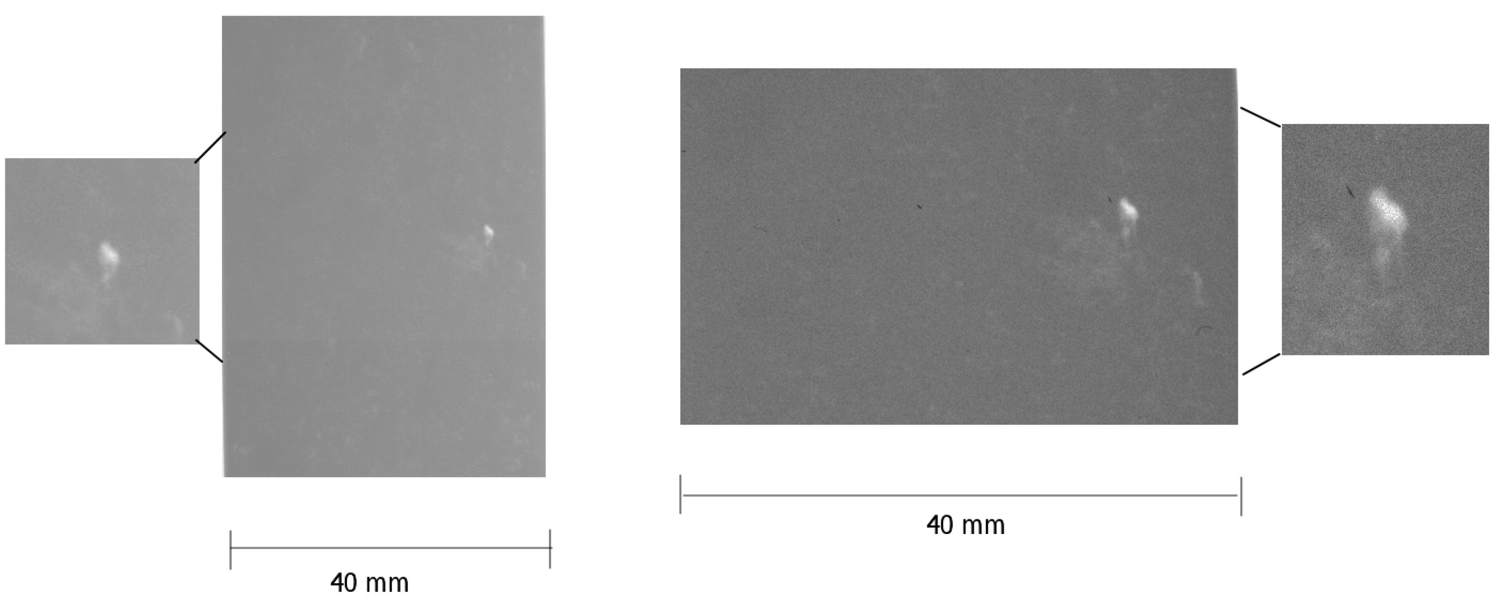
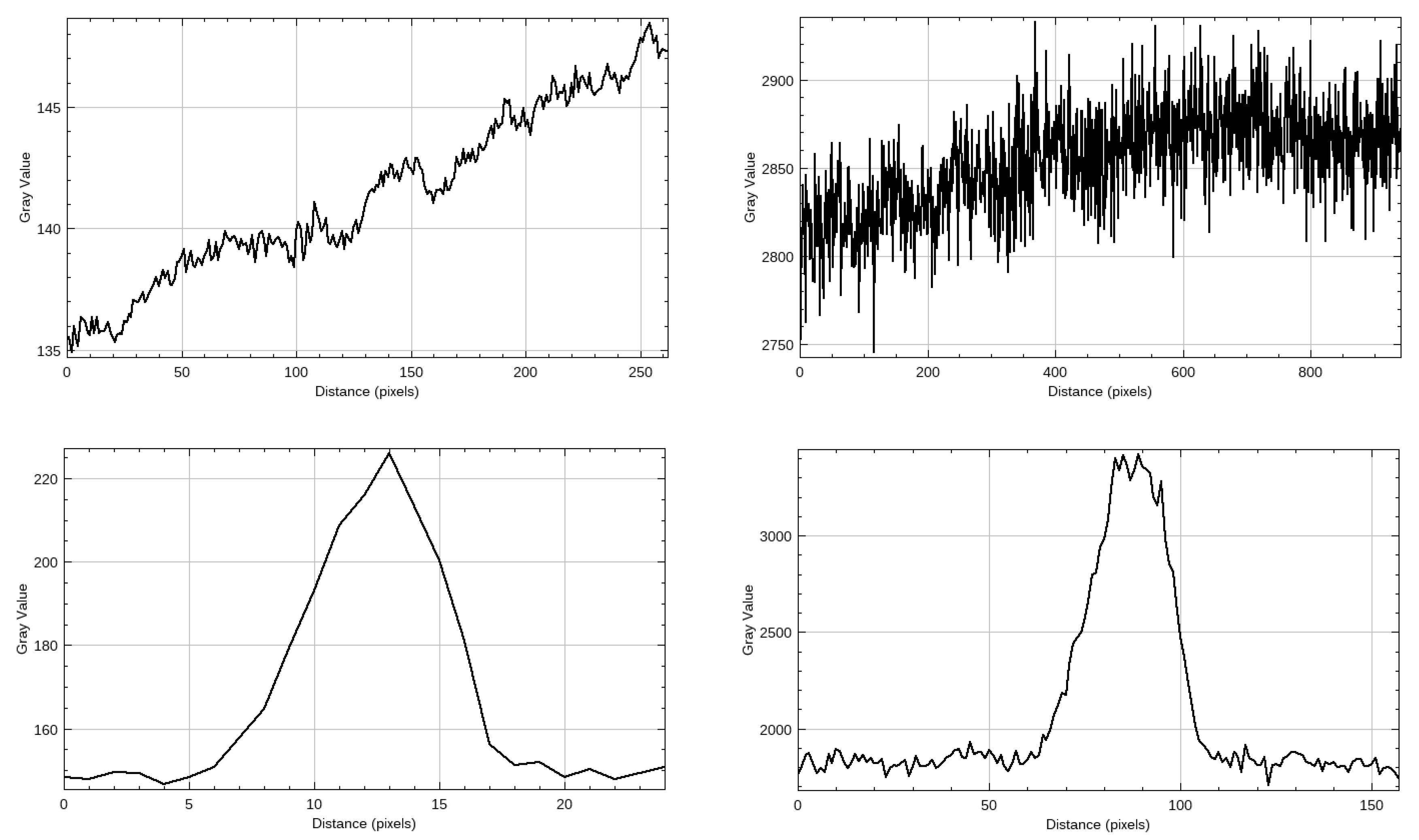
Samples of the original X-ray images are shown in Figure 9. The contrast of the pore peak is C(HighQ) = 1.42 and C(LowQ) = 1.86. The FWHM of the pore peak is FWHM(HighQ) = 7 px ≈ 0.7 mm and FWHM(LowQ) = 25 px ≈ 0.75 mm, as shown in Figure 10.

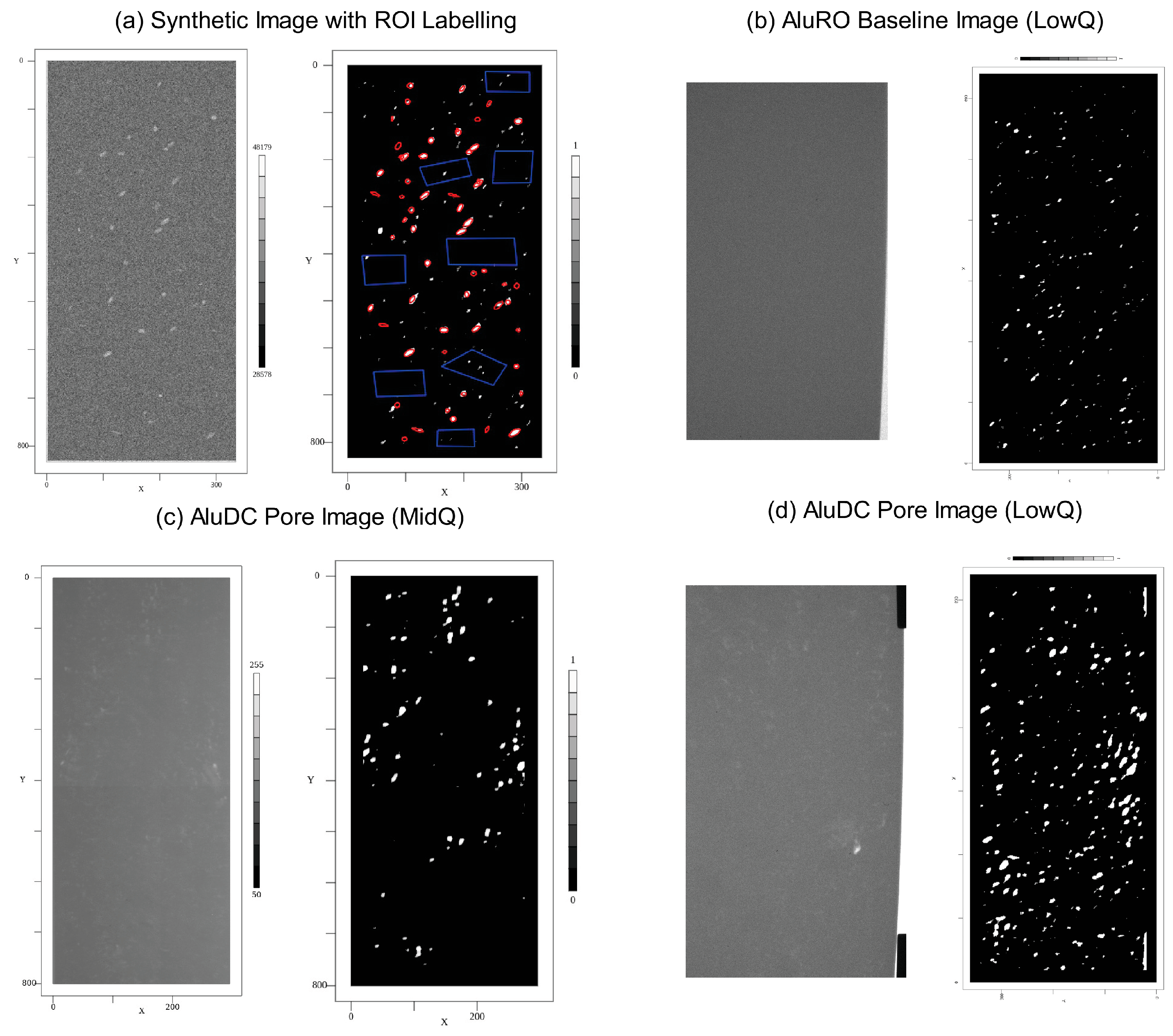
The main objective of this work was to apply a semantic pixel classifier for the feature marking of pores in aluminum die-casted plates using single projection X-ray images sampled using the LowQ device introduced in this paper. Since there is no ground truth in the measured images (i.e., accurate labeling for training is not possible), synthetic images retrieved from the numerical X-ray simulation were used to train the pixel classifier, which was finally applied to X-ray images thereafter.

Figure 11 shows some selected results. There are always image pairs consisting of the X-ray input image (left) and the pore feature-marking image (right), as predicted by the semantic pixel classifier. One of the synthetic images is shown in Figure 11a, as is the prediction of the trained model. Additionally, the feature image shows the ROI selection and labeling of the input images used for training (red: pore area; blue: selected background regions). The ROIs were automatically created from the CAD model used for simulation. The predictor model was trained with 40 epochs. The CNN architecture consists of two convolution-pooling layer pairs with 8 filters each. The training set consisted of an imbalanced set, with background examples being preferred to suppress false positive predictions rather than false negative. Since there is no ground truth for the measured images, we can only evaluate the results for the synthetic images. The overall accuracy achieved on the test set was 93%, with a class-specific error of 4% background and 11% pore region marking. The F1 score was 0.93. These results sound promising, and examples of the feature marking of the measured images are shown in Figure 11c,d for the low-noise Mid-Q and noisy Low-Q instruments, respectively. It can be seen that there is significantly increased pore feature marking in the LowQ images compared with the MidQ images. To estimate the impact of noise (from detector and radiation source), we tested a pore-free rolled and polished aluminum plate, as shown in Figure 11b, applying the same predictor model and expecting a black image; however, the image did not turn out to be black. This clearly shows the noise sensitivity of the predictor model, which must be suppressed. One approach for discriminating noise from pores in the feature marking of images is to calculate the union of two independent images from the same specimen, as it is expected (and can be shown) that noisy marking are randomly positioned. The geometric distortions of the Low-Q system seem to be irrelevant to the feature marking process.

6. Conclusions

One of the main findings of this work is that a low-cost constraint does not necessarily result in low-quality output (this applies to the LowQ device described in this work). With respect to resolution and contrast, the LowQ device outperforms an industrial MidQ device, but when using the LowQ device, the noise is significantly higher due to the lower overall sensitivity and long exposure times not allowing for the extra exposure required to significantly reduce image noise. Additionally, random popcorn/shot noise in the LowQ indirect imaging system requires at least two independent images to substantially remove this noise.

The higher noise of the LowQ instrument compared with the industrial MidQ device has a significant impact on the accuracy and quality of the data-driven, feature-marking model. The geometric distortions of the LowQ system seem to be irrelevant to the feature marking process. It was possible to train the feature-marking detector with pure synthetic X-ray images computed by a numerical simulator using a CAD model of the specimen with randomly created defects.

Future work must involve improving the training data set by overlaying measured noise (especially from the LowQ device) to the simulated X-ray images.