A Review of Mathematical Methods for the Evaluation of Defects in a Layered Specimen by Means of Active Thermography: Perturbation Theory, Linearization, and Reciprocity Gap ^†

Abstract

The thermal properties of a two-layered composite conductor are modified in the case that the interface is damaged. The present paper deals with the nondestructive evaluation of the perturbations of interface thermal conductance due to the presence of defects. The specimen was heated by means of a lamp system or a laser while its temperature was measured with an infrared camera in the typical framework of active thermography. The evaluation of the defects affecting the interface was made in the past using thin plate approximation or standard numerical techniques for inverse problems. Here, we show an explicit inversion formula obtained from the reciprocity property of parabolic equations.

1. Introduction

The thermal properties of a two-layered composite conductor are modified when the interface S is damaged. The present paper deals with the nondestructive evaluation of the thermal conductance of S in order to detect the presence of defects. The specimen was heated by means of a lamp system or a laser while its temperature was measured with an infrared camera in the typical framework of active thermography [1]. The mathematical (direct) model consists of a system of two Boundary Value Problems (BVPs) for the Laplace-transformed heat equation. In [2], defects affecting the interface were evaluated successfully by means of perturbation theory and thin plate approximation. An alternative strategy, based on reciprocity gap analysis is described here. A new inversion formula is shown in Section 4).

1.1. Layered Domains

We deal with a composite body made up of two thermally conducting layers divided by a very thin and microscopically irregular interspace filled up with air or other poorly conductive materials (let ${\kappa }_a$ be its thermal conductivity). As long as the specimen is heated by an external source, heat flows through the interspace mainly in correspondence to possible contact spots between the conducting layers. The effect of the interspace on the heat transfer between the two layers is usually modeled in terms of transmission conditions at a regular interface S that separates the conducting layers. Interfaces can be classified as perfect or imperfect according to their thermal properties [3]. Here, we deal with a Low-Conductivity Imperfect (LCI) interface, which allows for a temperature jump with continuous heat flux. The Thermal Contact Resistance (TCR) r is a non-negative parameter proportional to the temperature gap between the two sides of S. Its inverse $h=\frac{1}{r}$ is referred to as Thermal Contact Conductance (TCC). In LCI interfaces, the resistance is $r>>0$. In the limit case of infinite r, the interface is perfectly insulating and $h=0$. Here, we focus on the case in which the undamaged interface has a known constant (in space and time) TCC $h_{undam}=h_0$. The defect is thought to be a local perturbation of the interface between the layers. The occurrence of a similar defect produces locally a positive (in the case of damaged insulation) or negative (in the case of delamination, i.e., increased thermal contact resistance) change $\delta h$ in the TCC. There is no appreciable increase of the temperature gap between the opposite sides of S except on the damaged area, where we expect that the numerical value of $\frac{{\kappa }_a}{h_0+\delta h}$ gives a good approximation of the thickness of the damaged interface.

1.2. The Direct Model and the Inverse Problem

Assume that the lower layer ${\Omega }^{-}$ is heated from below by a lamp kept ON for ${\tau }_{max}$ seconds. Heat passes through the damaged interface S so that the temperature of ${\Omega }^{+}$ changes in time. Heat transfer through the interface is modeled by means of Robin transmission conditions (see, for example, [4]). Temperature maps $\psi (x,t)$ are taken, in the meantime, on the external surface of ${\Omega }^{+}$. It is remarkable that $\delta h$ is independent of time (at least in the time scale of ${\tau }_{max}$), so that it is convenient to apply Laplace’s transform to the equations and boundary conditions. In this way, we obtain a system of two BVPs for elliptic equations in ${\Omega }^{+}$ and ${\Omega }^{-}$ (connected by Robin transmission conditions) whose solutions $U^{+}$ and $U^{-}$ are the Laplace transform of the temperatures of the two layers. Our goal is to approximate $\delta h$ from the knowledge of the boundary thermal data referred to as incomplete because they are taken on the top side only.

2. Geometry in 2D, Notation, Direct Model, and Inverse Problem

Let $\Omega$ be the rectangle $(0,D)\times (-a^{-},a^{+})$ in the 2D space $(x,z)$.

Let ${\Omega }^{+}$ be $(0,D)\times (0,a^{+})$ and ${\Omega }^{-}$ be $(0,D)\times (-a^{-},0)$.

Let $S=\left\{\right(x,z)\phantom{a}s.t.\phantom{aa}0<x<Dandz=0\}$. Clearly, $\Omega ={\Omega }^{+}\cup S\cup {\Omega }^{-}$.

To fix the ideas, assume that $\frac{a^{+}+a^{-}}{D}<<1$. The geometry of the problem is summarized in Figure 1.

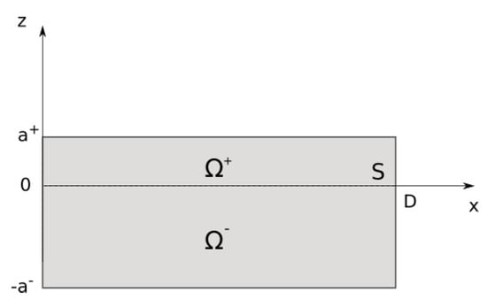
Figure 1. Geometrical scheme of the 2D specimen $\Omega$.

2.1. The Direct Model and the Interface Inverse Problem

The thermal behavior of each layer ${\Omega }^{\pm }$ is determined by its conductivity ${\kappa }^{\pm }$, density ${\rho }^{\pm }$, and specific heat $c^{\pm }$. Moreover, ${\alpha }^{\pm }=\frac{{\kappa }^{\pm }}{{\rho }^{\pm }{c}^{\pm }}$ denotes diffusivities. Heat transfer through the interface S depends on its thermal contact conductance $h\left(x\right)=h_0+\delta h\left(x\right)$. Let $u^{\pm }(x,z,t)$ with $(x,z)\in {\Omega }^{\pm }$ and $t>0$ the temperature increase (with respect to an initial and surrounding temperature $U_0$) in ${\Omega }^{\pm }$ obtained by applying, for a time interval $(0,t_{max})$, a heat flux $\varphi (x,t)$ to ${\Omega }^{-}$ (more precisely, $\varphi (x,t)=0$ for $t>t_{max}$). Clearly, $u(x,z,0)=0$. Assume that the vertical sides of the composite domain are insulated, while the horizontal sides exchange heat with the environment. The thermal contact conductances of the top ($z=a^{+}$) and bottom side ($z=-a^{-}$) are the positive constants $h^{+}$ and $h^{-}$, respectively. The constant parameters $a^{\pm }$, ${\kappa }^{\pm }$, ${\rho }^{\pm }$, $c^{\pm }$, and $h^{\pm }$ are known. When the interface thermal conductance $h\left(x\right)$ is given, the temperature $u^{\pm }$ fulfills a system of coupled Initial Boundary Value Problems (IBVPs) for the heat equation in the composite domain $\Omega$.

$${\rho }^{\pm }{c}^{\pm }{u}_t^{\pm }={\kappa }^{\pm }(u_{xx}^{\pm }+u_{zz}^{\pm }),(x,z)\in {\Omega }^{\pm },t>0$$

(1)

$$-{\kappa }^{-}{u}_z^{-}(x,-a^{-},t)+h^{-}{u}^{-}(x,-a^{-},t)=\varphi (x,t)and{\kappa }^{+}{u}_z^{+}(x,a^{+},t)+h^{+}{u}^{+}(x,a^{+},t)=0$$

(2)

with transmission conditions

$${\kappa }^{-}{u}_z^{-}(x,0,t)+h\left(x\right)\left[u\right](x,t)=0and{\kappa }^{-}{u}_z^{-}(x,0,t)={\kappa }^{+}{u}_z^{+}(x,0,t)$$

(3)

where $\left[u\right](x,t)=u^{-}(x,0,t)-u^{+}(x,0,t)$. It is $u_{\nu }^{\pm }=0$ on the vertical sides of ${\Omega }^{\pm }$, and the initial data are

$$u^{\pm }(x,z,0)=0,(x,z)\in {\Omega }^{\pm }.$$

(4)

Mathematical remark: If $\varphi$ and h are continuous functions and $H^1(\Omega )$ is a product Hilbert space equipped with a suitable norm, a unique solution $(u^{+},u^{-})\in L^2(0,T;H^1(\Omega ))$ exists, and it is stable with respect to variations of h (see [5]).

Interface inverse problem: If $\delta h\left(x\right)$ is unknown, we have the chance to approximate it from the knowledge of the flux $\varphi$ when the additional (boundary) dataset $\psi (x,t)=u^{+}(x,a^{+},t)$ for $t\in (0,t_{max})$ is available. This problem is closely related to the class of inverse heat conduction problems that are well known to be severely ill-posed (see [6]), hence the geometrical assumption that $\frac{a^{+}+a^{-}}{D}<<1$.

3. Thin Plate Approximation

System (1)–(4) is rewritten in normalized variables and expanded in powers of the thickness $\gamma =\frac{a_{+}}{D}$ of the slab. We get the second-order approximation:

$$h(x,y)\approx h_0(x,y)+{\gamma }^2{h}_1(x,y).$$

(5)

where the coefficients $h_0$ and $h_1$ are explicitly calculated in terms of the data $\Psi$ and $\Phi$ (details are given in [2], where (5) was successfully tested with real laboratory data).

4. Solution of the Inverse Problem by Means of Reciprocity Gap Equation

The unknown in our interface inverse problem is a perturbation $\delta h\left(x\right)$ of the original TCC $h_0$. Let $u_0^{\pm }$ be the background solution of (1)–(4) for $\delta h\left(x\right)\equiv 0$ and $u^{\pm }=u_0^{\pm }+\delta u^{\pm }$ the solution of (1)–(4) for $h=h_0+\delta h$. In the mathematical remark in Section 2.1, we observed that the direct model is well posed so that a small variation of the TCC determines a small variation of the temperature.

Along with [7,8,9], we applied the reciprocity principle for parabolic equations. Details about the following calculations are in [10]. First, we introduce the family:

$$v_n^{\pm }(x,z,t)=b_{\pm }{e}^{-At}{e}^{-s_{\pm }z}cos\left(\frac{2\pi }{D}nx\right)$$

(6)

$(n=0,1,2,...)$ of test functions (solutions of the backward heat equation) with $A>0$; $s^{\pm }=\sqrt{\frac{A}{{\alpha }^{\pm }}+p^2}$; $b_{+}=1$ and $b_{-}=\sqrt{\frac{A{\kappa }^{+}{\rho }^{+}{c}^{+}+{{\kappa }^{+}}^2{p}^2}{A{\kappa }^{-}{\rho }^{-}{c}^{-}+{{\kappa }^{-}}^2{p}^2}}$.

Plug the test functions into the reciprocity relation:

$${\int }_{TD}({\kappa }^{+}{v}_z^{+}(x,0,t)\left[u\right](x,t)+\left[v\right](x,t)(h_0+\delta \left(x\right))\left[u\right](x,t))\approx N$$

(7)

with

$$N={\int }_{TD}\{(-v^{+}{h}^{+}{u}^{+}-u^{+}{\kappa }^{+}{v}_z^{+})\left(a^{+}\right)-(v^{-}(h^{-}{u}^{-}-\varphi )+u^{-}{\kappa }^{-}{v}_z^{-})(-a^{-})\}.$$

(8)

Here, ${\int }_{TD}$ means ${\int }_0^{\infty }dt{\int }_0^{D}dx$. Then, apply Laplace’s transform and use the following heuristic linear expressions of $\left[\delta U\right]\left(x\right)={\int }_0^{\infty }{e}^{-At}\left[u\right](x,t)dt$ and $\delta U^{+}(x,0)={\int }_0^{\infty }{e}^{-At}\delta u^{+}$$(x,0,t)dt$ as functions of $\delta h$ (see the details in [10]):

$$\begin{array}{cc}\hfill \frac{\left[\delta U\right]\left(x\right)}{\left[U_0\right]}& \approx -E\delta h\left(x\right)\hfill \\ \hfill \frac{\delta U^{+}(x,0)}{\left[U_0\right]}& \approx E^{+}\delta h\left(x\right).\hfill \end{array}$$

(9)

with $E^{+}$ and E positive constants explicitly written in the Appendix of [10]. Finally, we get

$${\int }_0^D\widetilde{\delta h}cos\left(\frac{2\pi }{D}nx\right)dx\approx \frac{e^{-a^{+}{s}^{+}}(h^{+}-{\kappa }^{+}{s}^{+})}{h_0\left[U_0\right](1-h_{0}E-{\kappa }^{+}{s}^{+}{E}^{+})}{\int }_0^D\delta U^{+}(x,a^{+})cos\left(\frac{2\pi }{D}nx\right)dx$$

(10)

where $\widetilde{\delta h}\equiv \frac{\delta h}{h_0}$. Since the interface inverse problem is ill-posed, this reconstruction formula is expected to be unstable. However, it is possible to reduce the error magnification by means of a suitable choice of the Laplace’s frequency parameter A.

References

- Maldague, X. Nondestructive Evaluation of Materials by Infrared Thermography; Springer: New York, NY, USA, 1993. [Google Scholar]
- Scalbi, A.; Bozzoli, F.; Cattani, L.; Inglese, G.; Malavasi, M.; Olmi, R. Thermal imaging of inaccessible interfaces. Infrared Phys. Technol. 2022, 125, 104268. [Google Scholar] [CrossRef]
- Javili, A.; Kaessmair, S.; Steinmann, P. General Imperfect Interfaces. Comput. Methods Appl. Mech. Eng. 2014, 275, 76–97. [Google Scholar] [CrossRef]
- Cangiani, A.; Georgoulis, E.H.; Sabawi, Y.A. Adaptive discontinuous Galerkin methods for elliptic interface problems. Math. Comput. 2018, 87, 2675–2707. [Google Scholar] [CrossRef]
- Inglese, G.; Olmi, R. A note about the well-posedness of an Initial Boundary Value Problem for the heat equation in a layered domain. Rend. Ist. Mat. Univ. Trieste 2022, 54, 49–58. [Google Scholar] [CrossRef]
- Woodbury, K.A.; Najafi, H.; de Monte, F.; Beck, J.V. Inverse Heat Conduction: Ill-Posed Problems, 2nd ed.; Wiley: New York, NY, USA, 2023; ISBN 978-1-119-84019-0. [Google Scholar]
- Ben Abda, A.; Bui, H.D. Planar crack identification for the transient heat equation. J. Inverse Ill-Posed Probl. 2003, 11, 27–31. [Google Scholar] [CrossRef]
- Cakoni, F.; Cristo, M.D.; Sun, J. A multistep reciprocity gap functional method for the inverse problem in a multilayered medium. Complex Var. Elliptic Equ. 2012, 57, 261–276. [Google Scholar] [CrossRef]
- Colaco, M.J.; Alves, C.J.S. A Backward Reciprocity Function Approach to the Estimation of Spatial and Transient Thermal Contact Conductance in Double-Layered Materials Using Non-Intrusive Measurements. Numer. Heat Transf. Part A Appl. 2015, 68, 117–132. [Google Scholar] [CrossRef]
- Inglese, G. Formal derivation of an inversion formula for the approximation of interface defects by means of active thermography. arXiv 2023, arXiv:2309.04497. [Google Scholar] [CrossRef]
Disclaimer/Publisher’s Note: The statements, opinions and data contained in all publications are solely those of the individual author(s) and contributor(s) and not of MDPI and/or the editor(s). MDPI and/or the editor(s) disclaim responsibility for any injury to people or property resulting from any ideas, methods, instructions or products referred to in the content. |
© 2023 by the authors. Licensee MDPI, Basel, Switzerland. This article is an open access article distributed under the terms and conditions of the Creative Commons Attribution (CC BY) license (https://creativecommons.org/licenses/by/4.0/).