
Revisiting Structural Breaks in the Terms of Trade of Primary Commodities (1900–2020)—Markov Switching Models and Finite Mixture Distributions †


Abstract
:1. Introduction
2. A Finite Mixture Distributions Approach
2.1. Methodology
- K is the number of components,
- is the mixing weight of the ith component, is a normal component distribution of mean and variance .
- The specification of the number of components K,
- The component parameters and the weight distribution should be estimated from the data,Finally, we must assign each observation of the time series, , to a certain component of the mixture model by making inference on a hidden vector indicator .
- (1)
- Parameter simulation conditional on the classification :
- Sample the weights from a Dirichelet posterior ,
- Sample the variances in each group i, from an inverted Gamma distribution ,
- Sample the means in each group i, from an inverted Gamma distribution
- (2)
- Classification of each observation conditional on knowing ,
- RI is the estimator obtained by reciprocal importance sampling,
- IS is the estimator obtained by importance sampling,
- BS is the estimator obtained by bridge sampling techniques.
2.2. Results
2.2.1. The Choice of the Number of Components
2.2.2. The Parameters of the Mixture of Three Normal Distributions
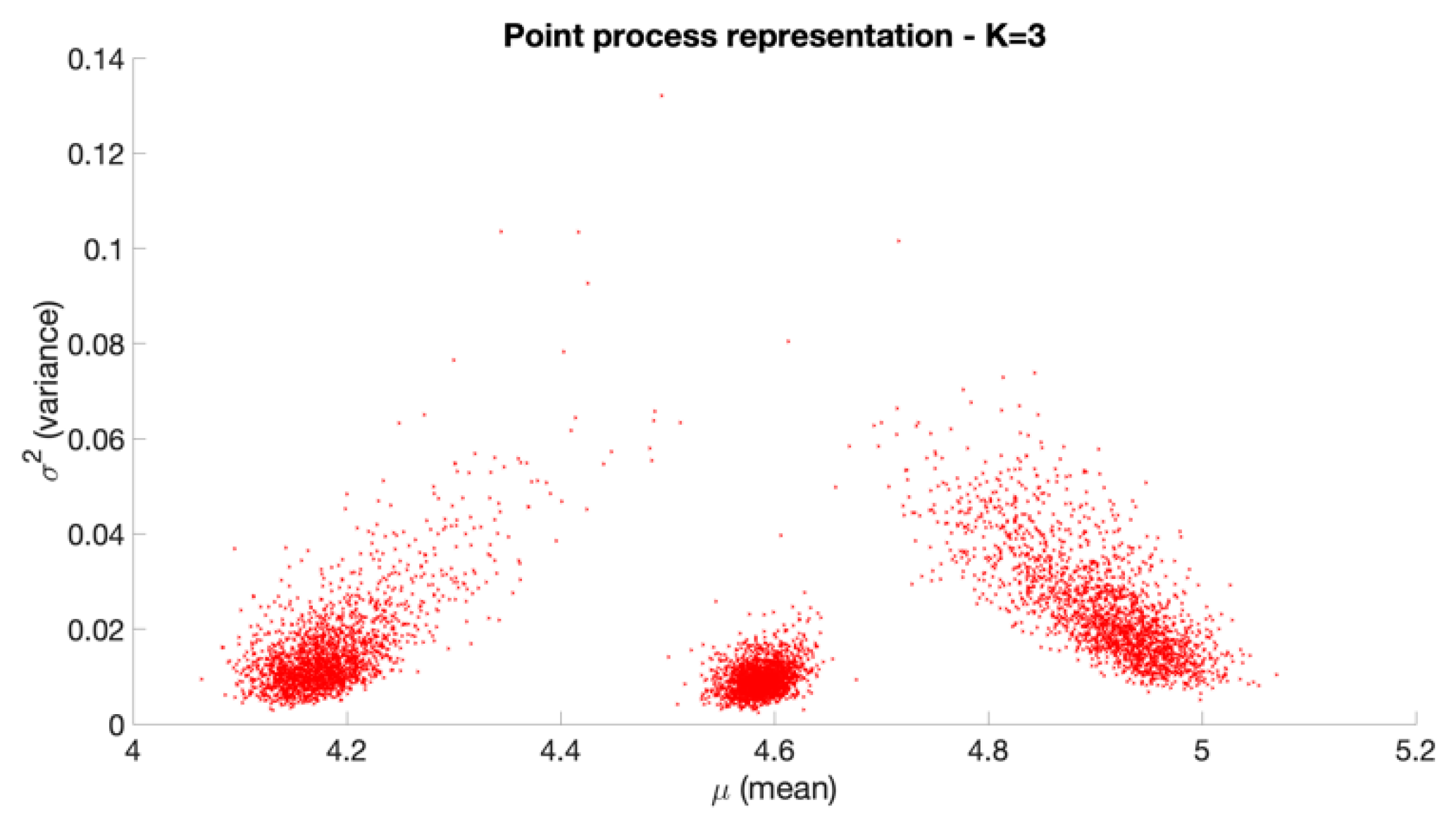
2.2.3. The Point Process Representation of Posterior Draws
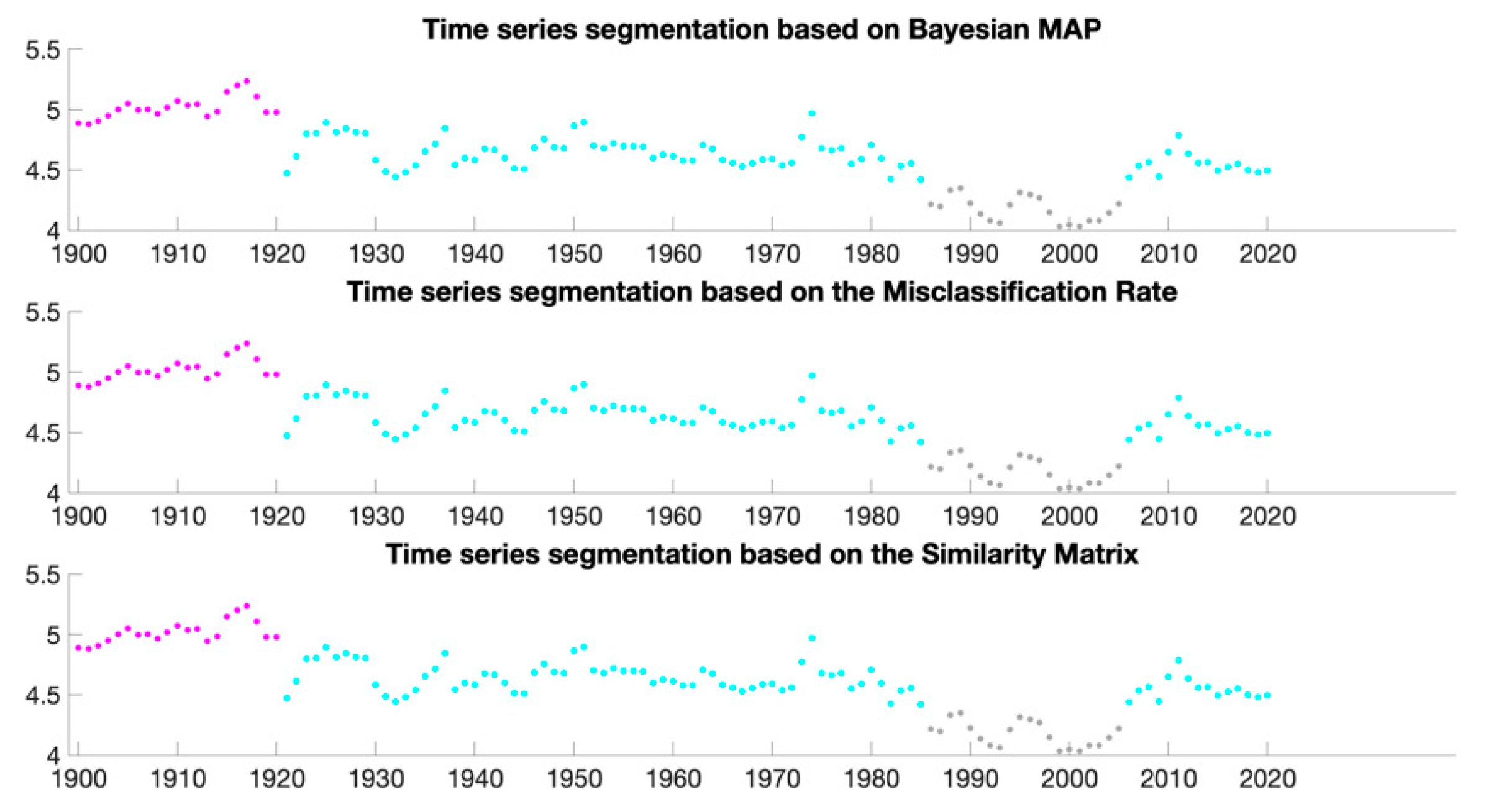
2.2.4. Clustering the Data
- The Bayesian maximum a posteriori (MAP),
- The similarity matrix based on the posterior similarity,
- The misclassification rate.
3. A Finite Markov Mixture Distributions Approach
3.1. Methodology
- for and .
3.2. Results
3.2.1. The Parameters of the Markov Mixture of Three Normal Distributions
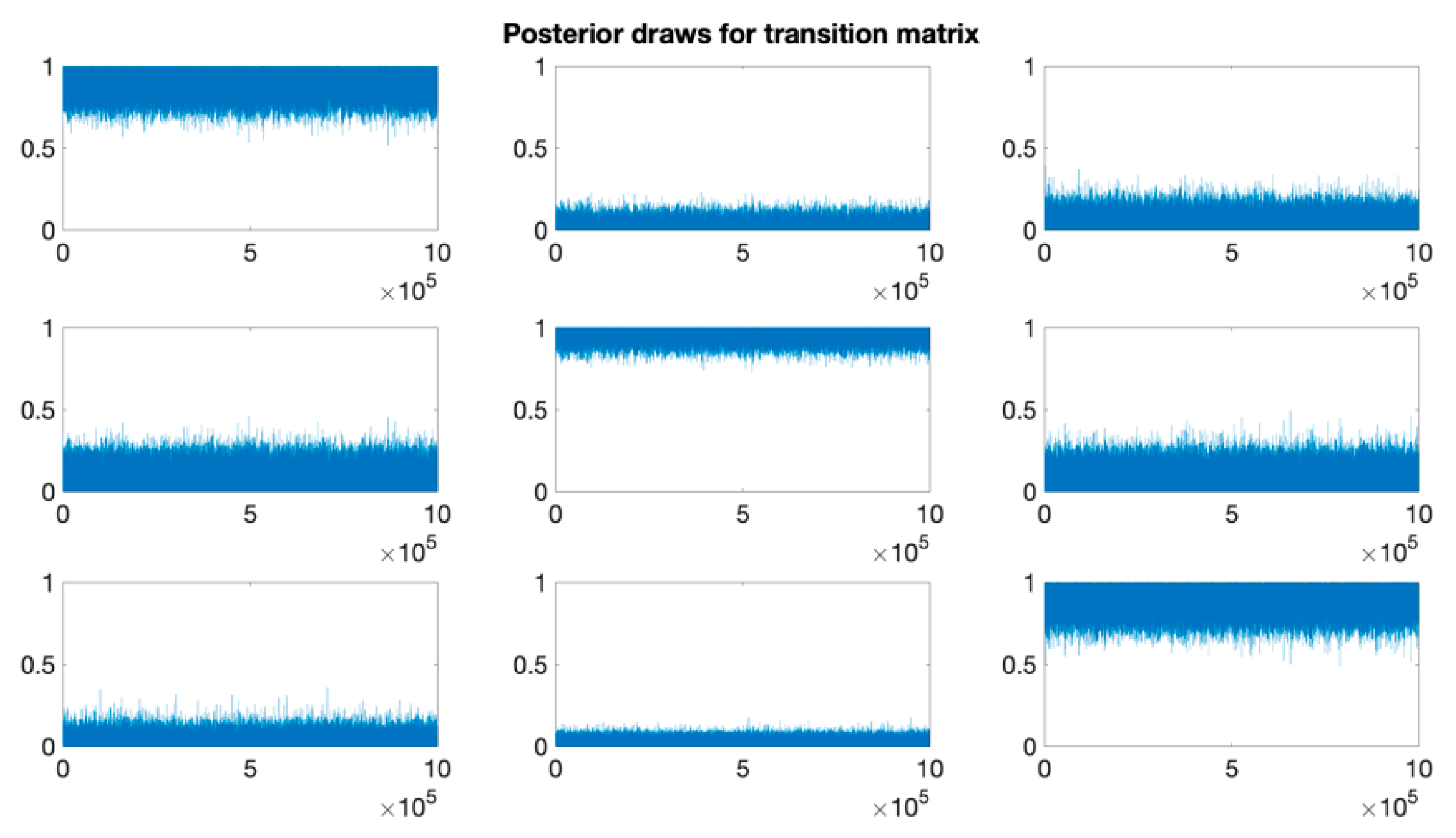
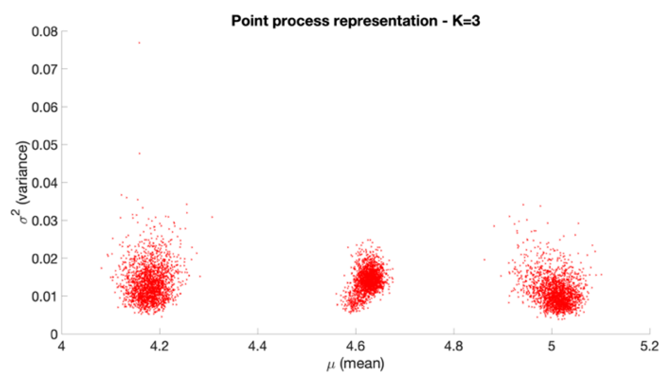
3.2.2. Point Process Representation of Posterior Draws
3.2.3. Clustering the Data
4. A Markov Switching Model Approach
4.1. Methodology
- denotes the series observed,
- are the independent regressors with fixed effects,
- are the independent regressors with random effects,
- these variables represent the autoregressive part of model,
- are independent variables with N (0, ) distribution,
- is modelled by a homogeneous Markov chain with K states.
- =, for and for i, j = 1, …, K (homogeneity of the chain).
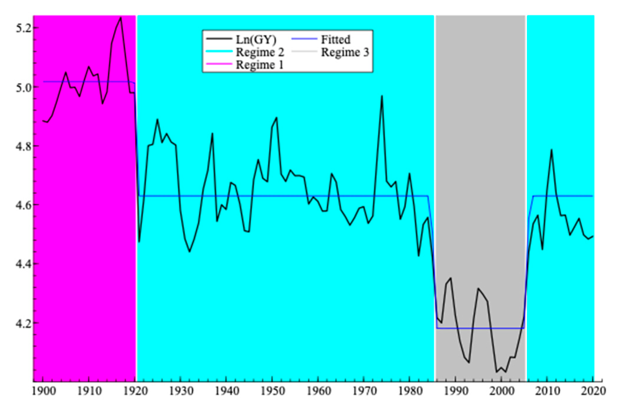
4.2. Results
5. Discussion and Conclusions
Institutional Review Board Statement
Informed Consent Statement
Data Availability Statement
References
- Prakash, A. Safeguarding Food Security in Volatile Global Markets; FAO: Rome, Italy, 2011. [Google Scholar]
- Geronimi, V.; Taranco, A. Revisiting the Prebisch-Singer hypothesis of a secular decline in the terms of trade of primary commodities (1900–2016). A dynamic regime approach. Resour. Policy 2018, 59, 329–339. [Google Scholar] [CrossRef]
- Prebisch, R. The Economic Development of Latin America and its Principal Problems. Econ. Bull. Lat. Am. 1962, 7, 1–22. [Google Scholar]
- Singer, H.W. U.S. Foreign Investment in Underdeveloped Areas: The distribution of gains between Investing and Borrowing countries. Am. Econ. Rev. Pap. Proc. 1950, 40, 473–485. [Google Scholar] [CrossRef]
- Grilli, E.R.; Yang, M.C. Primary commodity prices, manufactured goods prices, and the terms of trade of developing countries: What the long run shows. World Bank Econ. Rev. 1988, 2, 1–47. [Google Scholar] [CrossRef]
- Geronimi, V.; Anani, E.T.G.; Taranco, A. Notes on updating prices indices and terms of trade for primary commodities (No. 3–2017). Cahier CEMOTEV 2017, 2017, 3. [Google Scholar]
- Frühwirth-Schnatter, S. Finite Mixture and Markov Switching Models; Springer Series in Statistics; Springer: New York, NY, USA, 2006. [Google Scholar] [CrossRef]
- Celeux, G.; Frühwirth-Schnatter, S.; Robert, C.P. (Eds.) Handbook of Mixture Analysis; Chapman and Hall/CRC: Boca Raton, FL, USA, 2018. [Google Scholar] [CrossRef]
- Diebolt, J.; Robert, C. Bayesian Estimation of Finite Mixture Distributions, Part I: Theoretical Aspects; Rapport Technique LSTA; Université Paris VI: Paris, France, 1990; Volume 110. [Google Scholar]
- Robert, C.; Casella, G. A short history of Markov chain Monte Carlo: Subjective recollections from incomplete data. Stat. Sci. 2011, 26, 102–115. [Google Scholar] [CrossRef]
- Frühwirth-Schnatter, S. Keeping the balance—Bridge sampling for marginal likelihood estimation in finite mixture, mixture of experts and Markov mixture models. Braz. J. Probab. Stat. 2019, 33, 706–733. [Google Scholar] [CrossRef]
- Stephens, M. Bayesian analysis of mixture models with an unknown number of components-an alternative to reversible jump methods. Ann. Stat. 2000, 28, 40–74. [Google Scholar] [CrossRef]
- Hamilton, J.D. A new approach to the economic analysis of nonstationary time series and the business cycle. Econometrica 1989, 57, 357. [Google Scholar] [CrossRef]
- Hamilton, J.D. Regime-switching models. In Palgrave Dictionary of Economics; Durlauf, S., Blume, L., Eds.; Palgrave McMillan Ltd.: London, UK, 2005. [Google Scholar] [CrossRef] [Green Version]
- Dempster, A.P.; Laird, N.M.; Rubin, D.B. Maximum likelihood from incomplete data via the EM algorithm (with discussion). J. R. Statist. Soc. Ser. B 1977, 39, 1–38. [Google Scholar] [CrossRef] [Green Version]
- Lawrence, C.T.; Tits, A.L. A computationally efficient feasible sequential quadratic programming algorithm. Siam J. Optim. 2001, 11, 1092–1118. [Google Scholar] [CrossRef] [Green Version]


| Estimators | K = 1 | K = 2 | K = 3 | K = 4 | K = 5 |
|---|---|---|---|---|---|
| RI Standard error | −20.6488 8.2511 × 10⁻⁵ | −21.8398 1.0581 × 10⁻³ | −16.9335 3.2659 × 10⁻³ | −17.3682 6.9481 × 10⁻² | −21.2979 5.1914 × 10⁻¹ |
| IS Standard error | −20.6488 8.0611 × 10⁻⁵ | −21.8456 2.6576 × 10⁻³ | −16.9402 4.2801 × 10⁻³ | −17.1843 1.0072 × 10⁻¹ | −19.2823 1.199 × 10⁻¹ |
| BS Standard error | −20.6489 5.581 × 10⁻⁵ | −21.8402 7.2275 × 10⁻⁴ | −16.9316 9.0533 × 10⁻⁴ | −17.1489 2.4614 × 10⁻³ | −17.7954 6.2907 × 10⁻³ |
| Parameters of the kth Component | Distribution 1 | Distribution 2 | Distribution 3 |
|---|---|---|---|
| Weight | 0.3238 | 0.4945 | 0.1817 |
| Mean | 4.9091 | 4.5876 | 4.1829 |
| Standard deviation | 0.0246 | 0.0096 | 0.0153 |
| Distribution 1 | Distribution 2 | Distribution 3 | |
|---|---|---|---|
| Mean | 5.0099 | 4.6265 | 4.1822 |
| Standard deviation | 0.0110 | 0.0142 | 0.0134 |
| Regime 1, t | Regime 2, t | Regime 3, t | |
|---|---|---|---|
| Regime 1, t + 1 | 0.9384 | 0.0167 | 0.0284 |
| Regime 2, t + 1 | 0.0483 | 0.9637 | 0.0571 |
| Regime 3, t + 1 | 0.0133 | 0.0196 | 0.9146 |
| Regimes | Coefficient | Standard Error | t-Value | p-Value |
|---|---|---|---|---|
| Regime 1 | 5.01765 | 0.02014 | 249. | 0.000 |
| Regime 2 | 4.63002 | 0.01365 | 339. | 0.000 |
| Regime 3 | 4.18067 | 0.02514 | 166. | 0.000 |
| Regime 1, t | Regime 2, t | Regime 3, t | |
|---|---|---|---|
| Regime 1, t + 1 | 0.95451 | 0.0000 | 0.0000 |
| Regime 2, t + 1 | 0.045485 | 0.98722 | 0.048562 |
| Regime 3, t + 1 | 0.0000 | 0.012781 | 0.95144 |
Publisher’s Note: MDPI stays neutral with regard to jurisdictional claims in published maps and institutional affiliations. |
© 2021 by the authors. Licensee MDPI, Basel, Switzerland. This article is an open access article distributed under the terms and conditions of the Creative Commons Attribution (CC BY) license (https://creativecommons.org/licenses/by/4.0/).
Share and Cite
Taranco, A.; Geronimi, V. Revisiting Structural Breaks in the Terms of Trade of Primary Commodities (1900–2020)—Markov Switching Models and Finite Mixture Distributions. Eng. Proc. 2021, 5, 34. https://doi.org/10.3390/engproc2021005034
Taranco A, Geronimi V. Revisiting Structural Breaks in the Terms of Trade of Primary Commodities (1900–2020)—Markov Switching Models and Finite Mixture Distributions. Engineering Proceedings. 2021; 5(1):34. https://doi.org/10.3390/engproc2021005034
Chicago/Turabian StyleTaranco, Armand, and Vincent Geronimi. 2021. "Revisiting Structural Breaks in the Terms of Trade of Primary Commodities (1900–2020)—Markov Switching Models and Finite Mixture Distributions" Engineering Proceedings 5, no. 1: 34. https://doi.org/10.3390/engproc2021005034
APA StyleTaranco, A., & Geronimi, V. (2021). Revisiting Structural Breaks in the Terms of Trade of Primary Commodities (1900–2020)—Markov Switching Models and Finite Mixture Distributions. Engineering Proceedings, 5(1), 34. https://doi.org/10.3390/engproc2021005034