Kernel Two-Sample and Independence Tests for Nonstationary Random Processes ^†

Abstract

Two-sample and independence tests with the kernel-based mmd and hsic have shown remarkable results on i.i.d. data and stationary random processes. However, these statistics are not directly applicable to nonstationary random processes, a prevalent form of data in many scientific disciplines. In this work, we extend the application of mmd and hsic to nonstationary settings by assuming access to independent realisations of the underlying random process. These realisations—in the form of nonstationary time-series measured on the same temporal grid—can then be viewed as i.i.d. samples from a multivariate probability distribution, to which mmd and hsic can be applied. We further show how to choose suitable kernels over these high-dimensional spaces by maximising the estimated test power with respect to the kernel hyperparameters. In experiments on synthetic data, we demonstrate superior performance of our proposed approaches in terms of test power when compared to current state-of-the-art functional or multivariate two-sample and independence tests. Finally, we employ our methods on a real socioeconomic dataset as an example application.

1. Introduction

Nonstationary processes are the rule rather than the exception in many scientific disciplines such as epidemiology, biology, sociology, economics, or finance. In recent years, there has been a surge of interest in the analysis of problems described by large sets of interrelated variables with few observations over time, often involving complex nonlinear and nonstationary behaviours. Examples of such problems include the longitudinal spread of obesity in social networks [1], disease modelling from time-varying inter- and intracellular relationships [2], behavioural responses to losses of loved ones within social groups [3], and the linkage between climate change and the global financial system [4]. All such analyses rely on the statistical assessment of the similarity between, or the relationship amongst, noisy time series that exhibit temporal memory. Therefore, the ability to test the statistical significance of homogeneity and dependence between random processes that cannot be assumed to be independent and identically distributed (i.i.d.) is of fundamental importance in many fields.

Kernel-based methods provide a popular framework for homogeneity and independence tests by embedding probability distributions in rkhs [5] (Section 2.2). Of particular interest are the kernel-based two-sample statistic mmd (mmd) [6], which is used to assess whether two samples were drawn from the same distribution, hence testing for homogeneity; and the related hsic (hsic) [7], which is used to assess dependence between two random variables, thus testing for independence. These methods are nonparametric, i.e., they do not make any assumptions on the underlying distribution or the type of dependence. However, in their original form, both mmd and hsic assume access to a sample of i.i.d. observations—an assumption that is often violated for temporally-dependent data such as random processes.

Extensions of mmd and hsic to random processes have been proposed [8,9]. Yet, these methods require the random process to be stationary, meaning that its distribution does not change over time. While it is sometimes possible to approximately achieve stationarity with preprocessing techniques such as (seasonal) differencing or square root and power transformations, such approaches become cumbersome and notoriously difficult, particularly with large sets of variables. The stationarity assumption can therefore pose severe limitations in many application areas where multiple nonstationary processes must be taken into consideration. When studying the relationships of climate change to the global financial system, for example, factors such as greenhouse gas emissions, stock market indices, government spending, and corporate profits would have to be transformed or assumed to be stationary over time.

In this paper, we show how the kernel-based statistics mmd and hsic can be applied to nonstationary random processes. At the heart of our proposed approach is the simple, yet effective idea that realisations of a random process in the form of temporally-dependent measurements (i.e., the observed time series) can be viewed as independent samples from a multivariate probability distribution, provided that they are observed at the same points in time, i.e., over the same temporal grid. Then, mmd and hsic can be applied on these distributions to test for homogeneity and independence, respectively.

The remainder of this paper is structured as follows. After discussing related work in Section 2, we introduce our applications of two-sample and independence testing with mmd and hsic to nonstationary random processes in Section 3. We then carry out experiments on multiple synthetic datasets in Section 4 and demonstrate that the proposed tests have higher power compared with current functional or multivariate two-sample and independence tests under the same conditions. We provide an example application of our proposed methods to a socioeconomic dataset in Section 5 and conclude the paper with a brief discussion in Section 6.

2. Related Work

Two-sample and independence tests on stochastic processes have been widely studied in recent years. Under the stationarity assumption, ref. [8] investigate how the kernel cross-spectral density operator may be used to test for independence, and [9] formulate a wild bootstrap-based approach for both two-sample and independence tests, which outperforms [8] in various experiments. The wild bootstrap in [9] approximates the null hypothesis $H_0$ by assuming there exists a time lag $\tau$ such that a pair of measurements at any point in time t, ${(x_i,y_i)}_t$, is independent of ${(x_i,y_i)}_{t\pm s}$ for $s\ge \tau$. This method is applicable to test for instantaneous homogeneity and independence in stationary processes but requires further assumptions to investigate noninstantaneous cases: a maximum lag $M\le \tau$ must be defined as the largest absolute lag for the test. This results in multiple hypothesis testing requiring adjustment by a Bonferroni correction. Further, ref. [10] have applied distance correlation [11], a hsic-related statistic, to independence testing on stationary random processes.

Beyond the stationarity assumption, two-sample testing in the functional data analysis literature has mostly focused on differences of mean [12] or covariance structures [13,14]. However, ref. [15] have developed a two-sample test for distributions based on generalisations of a finite-dimensional test by utilising functional principal component analysis, and [16] have derived kernels over functions to be used with mmd for the two-sample test. Independence testing for functional data using kernels was recently proposed in [17] but assumes the samples lie on a finite-dimensional subspace of the function space—an assumption not required in our work. Moreover, ref. [18] have developed computationally efficient methods to test for independence on high-dimensional distributions and large sample sizes by using eigenvalues of centred kernel matrices to approximate the distribution under the null hypothesis $H_0$ instead of simulating a large number of permutations.

3. mmd and hsic for Nonstationary Random Processes

3.1. Notation and Assumptions

Let $\left\{{\mathbf{X}}_t\right\}$ and $\left\{{\mathbf{Y}}_t\right\}$ denote two nonstationary stochastic processes with probability laws ${\mathbb{P}}_{\mathbf{X}}$ and ${\mathbb{P}}_{\mathbf{Y}}$, respectively. We assume that we observe m independent realisations of $\left\{{\mathbf{X}}_t\right\}$ and n independent realisations of $\left\{{\mathbf{Y}}_t\right\}$ in the form of time series measured at $T_{\mathbf{X}}$ and $T_{\mathbf{Y}}$ time points, respectively. Said differently, the data samples $\mathbf{X}={\left\{{\mathbf{x}}_i\right\}}_{i=1}^m\stackrel{\mathrm{i}.\mathrm{i}.\mathrm{d}.}{\sim }{\mathbb{P}}_{\mathbf{X}}$ are a set of nonstationary time series, ${\mathbf{x}}_i=\{x_{i,1},\cdots ,x_{i,T_{\mathbf{X}}}\}$, arriving over the same temporal grid, and similarly for $\mathbf{Y}={\left\{{\mathbf{y}}_i\right\}}_{i=1}^n\stackrel{\mathrm{i}.\mathrm{i}.\mathrm{d}.}{\sim }{\mathbb{P}}_{\mathbf{Y}}$ with ${\mathbf{y}}_i=\{y_{i,1},\cdots ,y_{i,T_{\mathbf{Y}}}\}$. Note that the measurements $x_{i,t}$ and $y_{i,t}$ are not independent across time (we use the terms ‘sample’ and ‘realisation’ interchangeably to denote ${\mathbf{x}}_i$ and ${\mathbf{y}}_i$ and the term ’measurement’ to denote the temporally dependent vectors $x_{i,t}$ and $y_{i,t}$).

We may view the realisations ${\mathbf{x}}_i$ and ${\mathbf{y}}_i$ as samples of multivariate probability distributions of dimension $T_{\mathbf{X}}$ and $T_{\mathbf{Y}}$, respectively, which are independent at any given point in time, i.e., $x_{i,t}\perp \perp x_{j,t}$ and $y_{i,t}\perp \perp y_{j,t}$$\forall t$ and $\forall i\ne j$. Consequently, we can represent these distributions by their mean embeddings ${\mu }_{\mathbf{X}}$ and ${\mu }_{\mathbf{Y}}$ in reproducing kernel Hilbert space (rkhss) and use these to conduct kernel-based two-sample and independence tests. Given a characteristic kernel k, i.e., the mean embedding $\mu$ captures all information of a distribution $\mathbb{P}$ [19], the dependence between measurements in time is captured by the ordering of the variables, and the fact that any characteristic kernel k is injective, thus guaranteeing a unique mapping of any probability distribution into a rkhs [20].

For homogeneity testing (${\mathbb{P}}_{\mathbf{X}}\stackrel{?}{=}{\mathbb{P}}_{\mathbf{Y}}$), we use the kernel-based mmd statistic and require equal number of measurements $T=T_{\mathbf{X}}=T_{\mathbf{Y}}$ but allow different sample sizes, $m\ne n$. For independence testing (${\mathbb{P}}_{\mathbf{X}\mathbf{Y}}\stackrel{?}{=}{\mathbb{P}}_{\mathbf{X}}{\mathbb{P}}_{\mathbf{Y}}$), we employ the related hsic, and in this case number of measurements can differ, but we require the same number of realisations, $m=n$. We now describe how two-sample and independence tests can be performed under these assumptions.

3.2. mmd for Nonstationary Random Processes

Let $k:{\mathbb{R}}^T\times {\mathbb{R}}^T\to \mathbb{R}$ be a characteristic kernel, such as the Gaussian kernel $k(x,y)=exp(-\parallel x-y{\parallel }^2/{\sigma }^2)$, which uniquely maps ${\mathbb{P}}_{\mathbf{X}}$ and ${\mathbb{P}}_{\mathbf{Y}}$ to their associated rkhs ${\mathcal{H}}_k$ via the mean embeddings ${\mu }_{\mathbf{X}}:=\int k(\mathbf{x},·)d{\mathbb{P}}_{\mathbf{X}}\left(\mathbf{x}\right)$ and ${\mu }_{\mathbf{Y}}:=\int k(\mathbf{y},·)d{\mathbb{P}}_{\mathbf{Y}}\left(\mathbf{y}\right)$ [5] (Section 2.1). The mmd between ${\mathbb{P}}_{\mathbf{X}}$ and ${\mathbb{P}}_{\mathbf{Y}}$ in ${\mathcal{H}}_k$ is defined as [6]:

$${{\displaystyle \mathrm{MMD}}}^2({\mathcal{H}}_k,{\mathbb{P}}_{\mathbf{X}},{\mathbb{P}}_{\mathbf{Y}}):={\parallel {\mu }_{\mathbf{X}}-{\mu }_{\mathbf{Y}}\parallel }_{{\mathcal{H}}_k}^2\ge 0,\mathrm{with}\mathrm{equality}\mathrm{iff}{\mathbb{P}}_{\mathbf{X}}={\mathbb{P}}_{\mathbf{Y}}.$$

(1)

Given samples $\mathbf{X}$ and $\mathbf{Y}$, ${{\displaystyle \mathrm{MMD}}}^2({\mathcal{H}}_k,{\mathbb{P}}_{\mathbf{X}},{\mathbb{P}}_{\mathbf{Y}})$ can then be approximated by the following unbiased estimator [6]:

$${\widehat{{\displaystyle \mathrm{MMD}}}}_u^2({\mathcal{H}}_k,\mathbf{X},\mathbf{Y})=\sum _{i=1}^m\sum _{j\ne i}^m\frac{k({\mathbf{x}}_i,{\mathbf{x}}_j)}{m(m-1)}+\sum _{i=1}^n\sum _{j\ne i}^n\frac{k({\mathbf{y}}_i,{\mathbf{y}}_j)}{n(n-1)}-2\sum _{i=1}^m\sum _{j=1}^n\frac{k({\mathbf{x}}_i,{\mathbf{y}}_j)}{mn}.$$

(2)

Henceforth, we drop the implied ${\mathcal{H}}_k$ for ease of notation.

Using ${\widehat{{\displaystyle \mathrm{MMD}}}}_u^2(\mathbf{X},\mathbf{Y})$ as a test statistic, one can construct a statistical two-sample test for the null hypothesis $H_0:{\mathbb{P}}_{\mathbf{X}}={\mathbb{P}}_{\mathbf{Y}}$ against the alternative hypothesis $H_1:{\mathbb{P}}_{\mathbf{X}}\ne {\mathbb{P}}_{\mathbf{Y}}$ [21].

Let $\alpha$ be the significance level of the test, i.e., the maximum allowable probability of falsely rejecting $H_0$ and hence an upper bound on the type-I error. Given $\alpha$, the threshold $c_{\alpha }$ for the test statistic can be approximated with a permutation test as follows. We first generate P randomly permuted partitions of the set of all realisations $\mathbf{X}\cup \mathbf{Y}$ with sizes commensurate with $(\mathbf{X},\mathbf{Y})$, denoted $({\mathbf{X}}_p,{\mathbf{Y}}_p),p=1,\dots ,P$. We then compute ${\widehat{{\displaystyle \mathrm{MMD}}}}_u^2({\mathbf{X}}_p,{\mathbf{Y}}_p),\forall p$, and sort the results in descending order. Finally, we select the statistic at position $(1-\alpha )\times P$ as our empirical threshold ${\widehat{c}}_{\alpha }$. The null hypothesis $H_0$ is then rejected if ${\widehat{{\displaystyle \mathrm{MMD}}}}_u^2(\mathbf{X},\mathbf{Y})>{\widehat{c}}_{\alpha }$. For a computationally less expensive (but generally less accurate) option, the inverse cumulative density function of the Gamma distribution can be computed to approximate the null distribution [22].

3.3. hsic for Nonstationary Random Processes

Let ${\mathbb{P}}_{\mathbf{X}\mathbf{Y}}$ denote the joint distribution of $\left\{{\mathbf{X}}_t\right\}$ and $\left\{{\mathbf{Y}}_t\right\}$, and let ${\mathcal{H}}_k$ and ${\mathcal{G}}_l$ be separable rkhss with characteristic kernels $k:{\mathbb{R}}^{T_{\mathbf{X}}}\times {\mathbb{R}}^{T_{\mathbf{X}}}\to \mathbb{R}$ and $l:{\mathbb{R}}^{T_{\mathbf{Y}}}\times {\mathbb{R}}^{T_{\mathbf{Y}}}\to \mathbb{R}$, respectively. hsic is then defined as the mmd between ${\mathbb{P}}_{\mathbf{X}\mathbf{Y}}$ and ${\mathbb{P}}_{\mathbf{X}}{\mathbb{P}}_{\mathbf{Y}}$ [7]:

$$\begin{array}{cc}\hfill & {\displaystyle \mathrm{HSIC}}({\mathcal{H}}_k,{\mathcal{G}}_l,{\mathbb{P}}_{\mathbf{X}\mathbf{Y}}):={{\displaystyle \mathrm{MMD}}}^2{(}_k{\otimes }_l,{\mathbb{P}}_{\mathbf{X}\mathbf{Y}},{\mathbb{P}}_{\mathbf{X}}{\mathbb{P}}_{\mathbf{Y}})\hfill \\ \hfill & =\parallel {\mu }_{\mathbf{X}\mathbf{Y}}-{\mu }_{\mathbf{X}}\otimes {\mu }_{\mathbf{Y}}{\parallel }_{{}_k{\otimes }_l}^2\ge 0,\mathrm{with}\mathrm{equality}\mathrm{iff}{\mathbb{P}}_{\mathbf{X}\mathbf{Y}}={\mathbb{P}}_{\mathbf{Y}}{\mathbb{P}}_{\mathbf{Y}}.\hfill \end{array}$$

(3)

Here, ⊗ denotes the tensor product. Recall that we assume an equal number of realisations m for both processes, and let $\mathbf{K},\mathbf{L}\in {\mathbb{R}}^{m\times m}$ be the kernel matrices with entries $k_{ij}=k({\mathbf{x}}_i,{\mathbf{x}}_j)$ and $l_{ij}=l({\mathbf{y}}_i,{\mathbf{y}}_j)$, respectively. Given i.i.d. samples $(\mathbf{X},\mathbf{Y})$, an unbiased empirical estimator of ${\displaystyle \mathrm{HSIC}}({\mathcal{H}}_k,{\mathcal{G}}_l,{\mathbb{P}}_{\mathbf{X}\mathbf{Y}})$ is given by [23] (Theorem 2):

$${\widehat{{\displaystyle \mathrm{HSIC}}}}_u({\mathcal{H}}_k,{\mathcal{G}}_l,\mathbf{X}\mathbf{Y})=\frac{1}{m(m-3)}\left[\mathrm{trace}\left(\tilde{\mathbf{K}}\tilde{\mathbf{L}}\right)+\frac{{\mathbf{1}}^{\top }\tilde{\mathbf{K}}\mathbf{1}{\mathbf{1}}^{\top }\tilde{\mathbf{L}}\mathbf{1}}{(m-1)(m-2)}-\frac{2}{m-2}{\mathbf{1}}^{\top }\tilde{\mathbf{K}}\tilde{\mathbf{L}}\mathbf{1}\right],$$

(4)

where $\tilde{\mathbf{K}}=\mathbf{K}-\mathrm{diag}\left(\mathbf{K}\right)$ and $\tilde{\mathbf{L}}=\mathbf{L}-\mathrm{diag}\left(\mathbf{L}\right)$, and $\mathbf{1}$ is the $m\times 1$ vector of ones. To ease our notation, we henceforth omit the implied ${\mathcal{H}}_k$ and ${\mathcal{G}}_l$.

To test ${\widehat{{\displaystyle \mathrm{HSIC}}}}_u\left(\mathbf{X}\mathbf{Y}\right)$ for statistical significance, we define the null hypothesis $H_0:{\mathbb{P}}_{\mathbf{X}\mathbf{Y}}={\mathbb{P}}_{\mathbf{X}}{\mathbb{P}}_{\mathbf{Y}}$ and the alternative $H_1:{\mathbb{P}}_{\mathbf{X}\mathbf{Y}}\ne {\mathbb{P}}_{\mathbf{X}}{\mathbb{P}}_{\mathbf{Y}}$. We broadly repeat the procedure outlined in Section 3.2 by bootstrapping the distribution under $H_0$ via permutations, with the distinction that we only permute the samples ${\left\{{\mathbf{y}}_i\right\}}_{i=1}^m$, resulting in ${\mathbf{Y}}_p,p\in [1,P]$, whilst the ${\left\{{\mathbf{x}}_j\right\}}_{j=1}^m$ are kept unchanged [7]. ${\widehat{{\displaystyle \mathrm{HSIC}}}}_u\left(\mathbf{X}\mathbf{Y}\right)$ is then computed for each permutation $(\mathbf{X},{\mathbf{Y}}_p)$ and the empirical threshold ${\widehat{c}}_{\alpha }$ is taken as the statistic at position $(1-\alpha )\times P$. The null hypothesis $H_0$ is rejected, if ${\widehat{{\displaystyle \mathrm{HSIC}}}}_u\left(\mathbf{X}\mathbf{Y}\right)>{\widehat{c}}_{\alpha }$.

3.4. Maximising the Test Power

The power of both mmd-based two-sample and hsic-based independence tests is prone to decay in high dimensional spaces [24,25], as in our setting where each measurement point in time is treated as a separate dimension. Hence, we describe here how a kernel k can be chosen to maximise the test power, i.e., the probability of correctly rejecting $H_0$ given that it is false. First, note that under $H_1$ both ${\widehat{{\displaystyle \mathrm{MMD}}}}_u^2(\mathbf{X},\mathbf{Y})$ [21] (Corollary 16) and ${\widehat{{\displaystyle \mathrm{HSIC}}}}_u\left(\mathbf{X}\mathbf{Y}\right)$ [7] (Theorem 1) are asymptotically Gaussian:

$$\begin{array}{cc}\hfill \frac{{\widehat{{\displaystyle \mathrm{MMD}}}}_u^2(\mathbf{X},\mathbf{Y})-{{\displaystyle \mathrm{MMD}}}^2({\mathbb{P}}_{\mathbf{X}},{\mathbb{P}}_{\mathbf{Y}})}{\sqrt{V_m^{{\displaystyle \mathrm{MMD}}}({\mathbb{P}}_{\mathbf{X}},{\mathbb{P}}_{\mathbf{Y}})}}& \stackrel{D}{⟶}\mathcal{N}(0,1)\hfill \end{array}$$

(5)

$$\begin{array}{cc}\hfill \frac{{\widehat{{\displaystyle \mathrm{HSIC}}}}_u\left(\mathbf{X}\mathbf{Y}\right)-{\displaystyle \mathrm{HSIC}}\left({\mathbb{P}}_{\mathbf{X}\mathbf{Y}}\right)}{\sqrt{V_m^{{\displaystyle \mathrm{HSIC}}}({\mathbb{P}}_{\mathbf{X}\mathbf{Y}}})}& \stackrel{D}{⟶}\mathcal{N}(0,1),\hfill \end{array}$$

(6)

where $V_m^{{\displaystyle \mathrm{MMD}}}({\mathbb{P}}_{\mathbf{X}},{\mathbb{P}}_{\mathbf{Y}})$ and $V_m^{{\displaystyle \mathrm{HSIC}}}\left({\mathbb{P}}_{\mathbf{X}\mathbf{Y}}\right)$ denote the asymptotic variance of ${\widehat{{\displaystyle \mathrm{MMD}}}}_u^2(\mathbf{X},\mathbf{Y})$ and ${\widehat{{\displaystyle \mathrm{HSIC}}}}_u\left(\mathbf{X}\mathbf{Y}\right)$, respectively [26] (Section 5.5.1 (A)).

Given a significance level $\alpha$, we define the test thresholds $c_{\alpha }^{{\displaystyle \mathrm{MMD}}}$ and $c_{\alpha }^{{\displaystyle \mathrm{HSIC}}}$ and reject $H_0$ if ${\widehat{{\displaystyle \mathrm{MMD}}}}_u^2(\mathbf{X},\mathbf{Y})>c_{\alpha }^{{\displaystyle \mathrm{MMD}}}$ or ${\widehat{{\displaystyle \mathrm{HSIC}}}}_u\left(\mathbf{X}\mathbf{Y}\right)>c_{\alpha }^{{\displaystyle \mathrm{HSIC}}}$. Following [27], the test power is defined in terms of ${\mathbb{P}}_1$, the distributions under $H_1$, with equal sample sizes $m=n$ as:

$$\begin{array}{cc}\hfill {\mathbb{P}}_1\left({\widehat{{\displaystyle \mathrm{MMD}}}}_u^2(\mathbf{X},\mathbf{Y})>\frac{{\widehat{c}}_{\alpha }^{{\displaystyle \mathrm{MMD}}}}{m}\right)& \stackrel{D}{⟶}\Phi \left(\frac{{{\displaystyle \mathrm{MMD}}}^2({\mathbb{P}}_{\mathbf{X}},{\mathbb{P}}_{\mathbf{Y}})-c_{\alpha }^{{\displaystyle \mathrm{MMD}}}/m}{\sqrt{V_m^{{\displaystyle \mathrm{MMD}}}({\mathbb{P}}_{\mathbf{X}},{\mathbb{P}}_{\mathbf{Y}})}}\right)\hfill \end{array}$$

(7)

$$\begin{array}{cc}\hfill {\mathbb{P}}_1\left({\widehat{{\displaystyle \mathrm{HSIC}}}}_u\left(\mathbf{X}\mathbf{Y}\right)>\frac{{\widehat{c}}_{\alpha }^{{\displaystyle \mathrm{HSIC}}}}{m}\right)& \stackrel{D}{⟶}\Phi \left(\frac{{\displaystyle \mathrm{HSIC}}\left({\mathbb{P}}_{\mathbf{X}\mathbf{Y}}\right)-c_{\alpha }^{{\displaystyle \mathrm{HSIC}}}/m}{\sqrt{V_m^{{\displaystyle \mathrm{HSIC}}}\left({\mathbb{P}}_{\mathbf{X}\mathbf{Y}}\right)}}\right),\hfill \end{array}$$

(8)

where $\Phi$ is the cumulative density function of the standard Gaussian distribution and where ${\widehat{c}}_{\alpha }\to c_{\alpha }$ with increasing sample size. To maximise the test power, we maximise the argument of $\Phi$, which we approximate by maximising ${\widehat{{\displaystyle \mathrm{MMD}}}}_u^2(\mathbf{X},\mathbf{Y})/\sqrt{{\widehat{V}}_m^{{\displaystyle \mathrm{MMD}}}(\mathbf{X},\mathbf{Y})}$ and minimising ${\widehat{c}}_{\alpha }^{{\displaystyle \mathrm{MMD}}}/\left(m\sqrt{{\widehat{V}}_m^{{\displaystyle \mathrm{MMD}}}(\mathbf{X},\mathbf{Y})}\right)$ for (7), and similarly for (8). The empirical unbiased variance ${\widehat{V}}_m^{{\displaystyle \mathrm{MMD}}}(\mathbf{X},\mathbf{Y})$ in (7) was derived in [27], and we use [23] (Theorem 5) for ${\widehat{V}}_m^{\mathrm{HSIC}}\left(\mathbf{X}\mathbf{Y}\right)$ in (8).

We perform this optimisation by splitting our samples $(\mathbf{X},\mathbf{Y})$ into training and testing sets, of which we take the former to learn the kernel hyperparameters and the latter to conduct the final hypothesis test with the learnt kernel.

4. Experimental Results on Synthetic Data

To evaluate our proposed tests empirically, we first apply our homogeneity and independence tests to various nonstationary synthetic datasets. We report test performance using $\widehat{\mu }$, the percentage of rejection of the null hypothesis $H_0$, which becomes the test power once $H_0$ is false, by repeating the experiments on 200 trials (i.e., 200 independently generated synthetic datasets). We provide $95\%$ confidence intervals computed as $\widehat{\mu }\pm 1.96\sqrt{\widehat{\mu }(1-\widehat{\mu })/200}$.

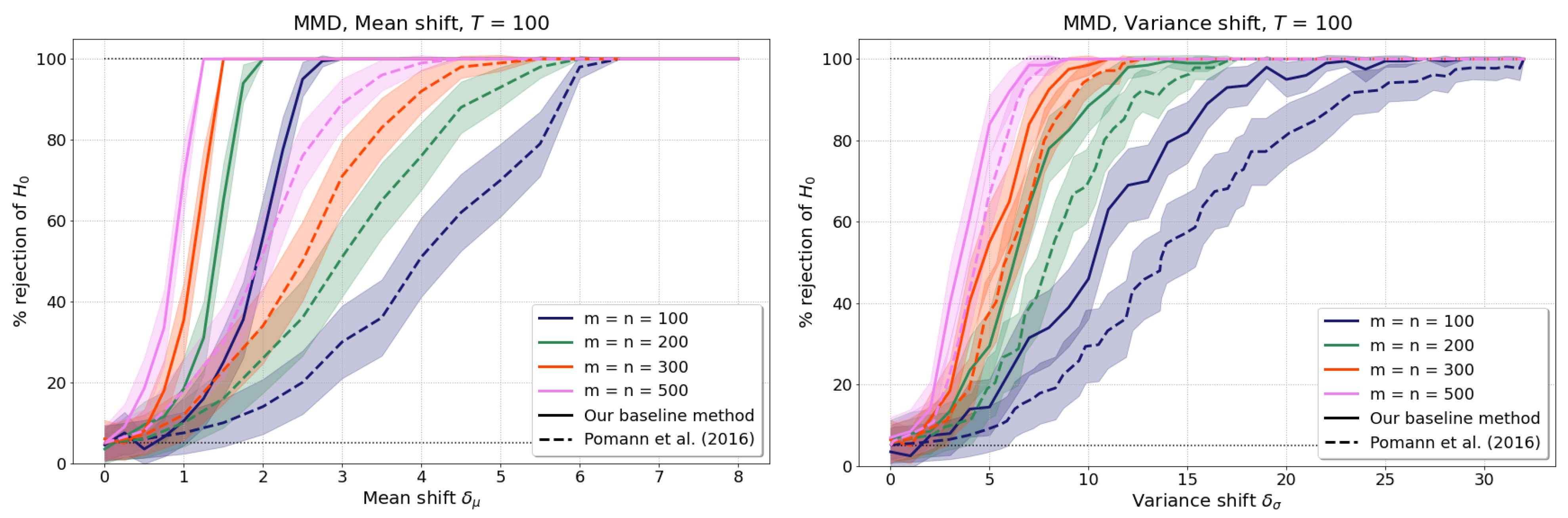
4.1. Homogeneity Tests with mmd

4.1.1. Setup

We evaluate our mmd-based homogeneity test against shifts in mean and variance of two nonstationary stochastic processes $\left\{{\mathbf{X}}_t\right\}$ and $\left\{{\mathbf{Y}}_t\right\}$ by establishing if they are correctly accepted or rejected under the null hypothesis $H_0:{\mathbb{P}}_{\mathbf{X}}={\mathbb{P}}_{\mathbf{Y}}$. For ease of comparison, we adopt the experimental protocol of [15] and consider two stochastic processes based on a linear mixed effects model. We generate independent samples $\mathbf{X}={\left\{{\mathbf{x}}_i\right\}}_{i=1}^m$ and $\mathbf{Y}={\left\{{\mathbf{y}}_i\right\}}_{i=1}^n$ on an equally spaced temporal grid of length $T_{\mathbf{X}}=T_{\mathbf{Y}}=T$ in the interval $\mathcal{I}=[0,1]$,

$$\begin{array}{cc}\hfill x_{i,t}& ={\mu }_{\mathbf{X}}\left(t\right)+\sum _{k=1}^K{{\xi }_{\mathbf{X}}}_{i,k}{\varphi }_k\left(t\right)+{{ϵ}_{\mathbf{X}}}_{i,t}\mathrm{and}{y}_{i,t}={\mu }_{\mathbf{Y}}\left(t\right)+\sum _{k=1}^K{{\xi }_{\mathbf{Y}}}_{i,k}{\varphi }_k\left(t\right)+{{ϵ}_{\mathbf{Y}}}_{i,t},\hfill \end{array}$$

(9)

where we set $K=2$ with Fourier basis functions ${\varphi }_1\left(t\right)=\sqrt{2}sin\left(2\pi t\right)$ and ${\varphi }_2\left(t\right)=\sqrt{2}cos\left(2\pi t\right)$. The coefficients ${{\xi }_{\mathbf{X}}}_{i,k}$ and ${{\xi }_{\mathbf{Y}}}_{i,k}$ and the additive noises ${{ϵ}_{\mathbf{X}}}_{i,t},{{ϵ}_{\mathbf{Y}}}_{i,t}$ are all independent Gaussian-distributed random variables with means and variances specified below.

We evaluate the test power against varying values of shifts in mean and variance as follows:

• Mean shift:${\mu }_{\mathbf{X}}\left(t\right)=t$ and ${\mu }_{\mathbf{Y}}\left(t\right)=t+{\delta }_{\mu }{t}^3$. The basis coefficients are sampled as ${{\xi }_{\mathbf{X}}}_{i,1},{{\xi }_{\mathbf{Y}}}_{i,1}\sim \mathcal{N}(0,10)$ and ${{\xi }_{\mathbf{X}}}_{i,2},{{\xi }_{\mathbf{Y}}}_{i,2}\sim \mathcal{N}(0,5)$, and the additive noises are sampled as ${{ϵ}_{\mathbf{X}}}_{i,t},{{ϵ}_{\mathbf{Y}}}_{i,t}\sim \mathcal{N}(0,0.25)$.
• Variance shift: We take ${\mu }_{\mathbf{X}}\left(t\right)={\mu }_{\mathbf{Y}}\left(t\right)=0$, and introduce a shift in variance in the first basis function coefficients via ${{\xi }_{\mathbf{X}}}_{i,1}\sim \mathcal{N}(0,10)$ and ${{\xi }_{\mathbf{Y}}}_{i,1}\sim \mathcal{N}(0,10+{\delta }_{\sigma })$. The second coefficients are sampled as ${{\xi }_{\mathbf{X}}}_{i,2},{{\xi }_{\mathbf{Y}}}_{i,2}\sim \mathcal{N}(0,5)$, and the noises as ${{ϵ}_{\mathbf{X}}}_{i,t},{{ϵ}_{\mathbf{Y}}}_{i,t}\sim \mathcal{N}(0,0.25)$.

The coefficients ${\delta }_{\mu }$ and ${\delta }_{\sigma }$ for mean and variance shifts, respectively, determine the departure from the null hypothesis. Setting ${\delta }_{\mu },{\delta }_{\sigma }=0$ means $H_0$ is true, whereas ${\delta }_{\mu },{\delta }_{\sigma }>0$ means $H_0$ is false. Although this is not a necessity, we set the number of independent samples of $\left\{{\mathbf{X}}_t\right\}$ and $\left\{{\mathbf{Y}}_t\right\}$ to be equal, $m=n$. To test for statistical significance, we follow the procedure described in Section 3.2 and perform permutation tests of $P=5000$ partitions for varying values of ${\delta }_{\mu }$ and ${\delta }_{\sigma }$ and different sample sizes $m=100,200,300,500$.

4.1.2. Baseline Results without Test Power Optimisation

Our baseline results are obtained with a Gaussian kernel $k(x,y)=exp(-\parallel x-y{\parallel }^2/{\sigma }^2)$ with bandwidth $\sigma$ equal to the median distance between observations of the aggregated samples. Figure 1 shows how our method (solid lines) compares to [15] (dashed lines) for $T=100$ discrete time points. For all sample sizes, the type-I error rate lies at or below the allowable probability of false rejection $\alpha$, and our method significantly outperforms [15] for nearly all levels of mean and variance shifts. Both shifts become easier to detect for larger sample sizes. Particularly strong improvements are achieved for mean shifts: our method makes no type-II errors for ${\delta }_{\mu }\ge 3$ on $m=100$ samples, whereas [15] only reach such performance with $m=500$ samples and ${\delta }_{\mu }\ge 4.5$. We obtain similar test power results (see Appendix A.1) for coarser realisations with $T=5,10,25,50$ over the same interval $\mathcal{I}=[0,1]$.

Figure 1. Results of our mmd-based homogeneity test for nonstationary random processes: percentage of rejected $H_0$ as mean shift (left) and variance shift (right) are varied. Our baseline method (solid lines) is compared to [15] (dashed lines) for different sample sizes $m=n=100,200,300,500$ and $T=100$ discrete time points.

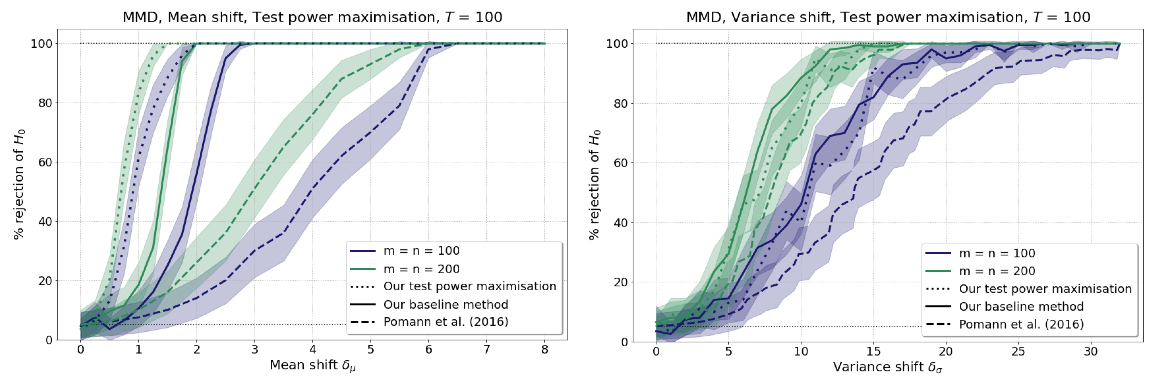
4.1.3. Results of the Optimised Test

Next, we apply the method described in Section 3.4 to maximise the test power. Specifically, we search for the Gaussian kernel bandwidth $\sigma$ (over spaces defined in Table A1 in Appendix A.2), that maximises the argument of $\Phi$ in our approximations of (7) on our training samples. For demonstrative purposes, we choose to split our dataset equally into training and testing sets although other ratios may lead to higher test power. Figure 2 shows the results of the optimised test (dotted lines) against the baseline results (solid lines) and the results of [15] (dashed lines) for $m=100$ and $m=200$ samples and $T=100$ discrete points in time. We find that the test power is significantly improved by our optimisation for the detection of mean shifts. For instance, test power rises fourfold for ${\delta }_{\mu }=1$ and $m=200$ compared to our baseline method. Furthermore, we have no type-II errors once ${\delta }_{\mu }\ge 2$ for $m=100$, as compared to ${\delta }_{\mu }\ge 3$ for our baseline test and ${\delta }_{\mu }\ge 6.5$ for [15]. In its current form, however, our optimisation does not yield higher test power for the detection of variance shifts, a fact that we discuss in Section 6.

Figure 2. Results of homogeneity test with optimising for test power: percentage of rejected $H_0$ for mean shift (left) and variance shift (right) for sample sizes $m=n=100,200$ and $T=100$ discrete time points. Our optimised test power method (dotted lines) is compared to our baseline method (solid lines) and [15] (dashed lines).

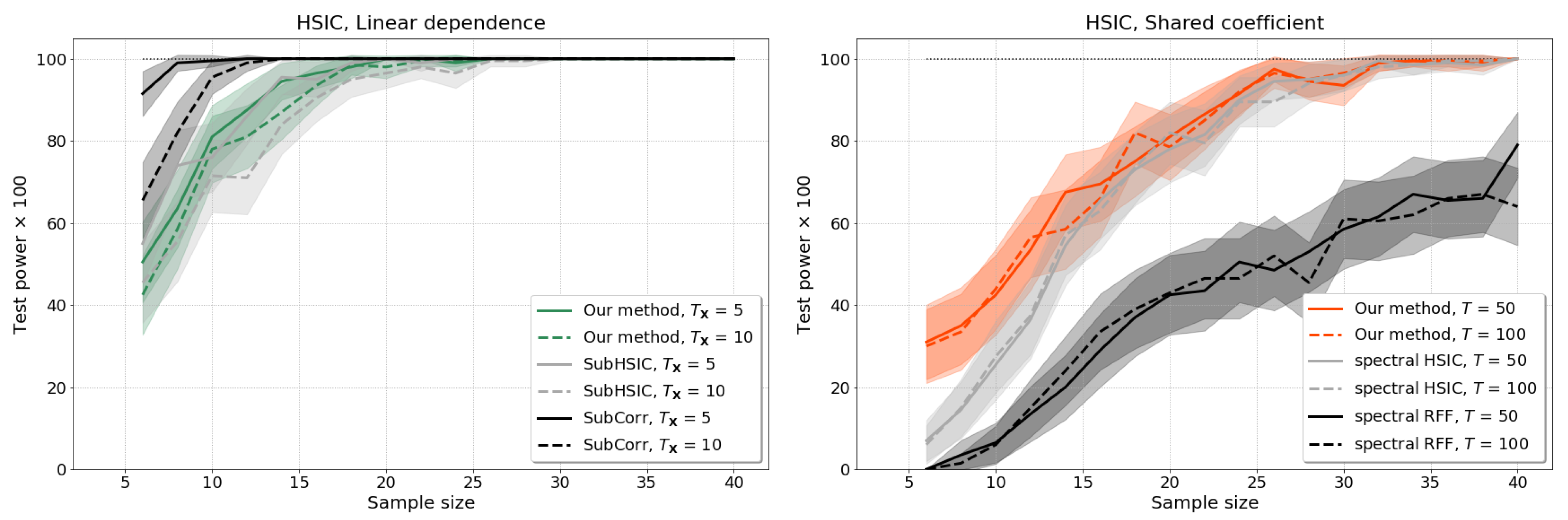
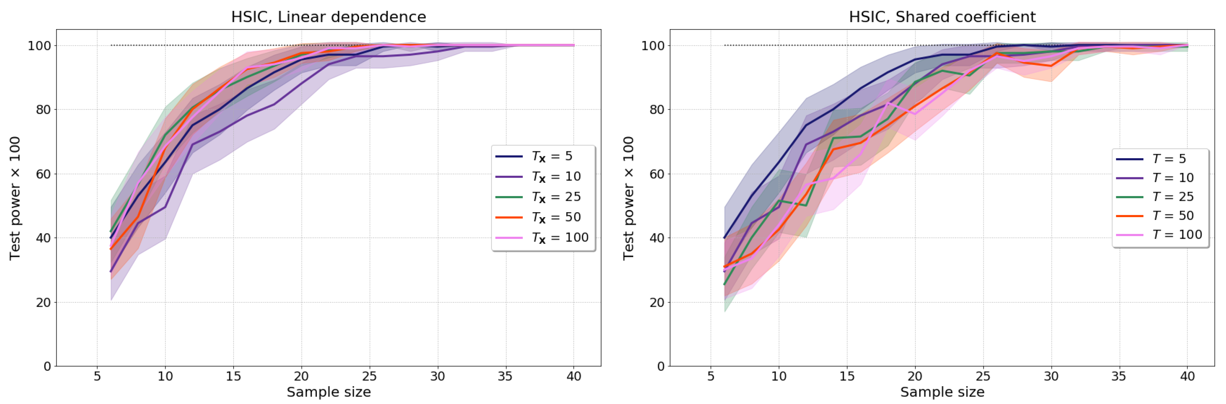
4.2. Independence Tests with hsic

4.2.1. Setup

To test for independence, the null hypothesis is $H_0:{\mathbb{P}}_{\mathbf{XY}}={\mathbb{P}}_{\mathbf{X}}{\mathbb{P}}_{\mathbf{Y}}$. We assume we observe measurements $x_{i,t}$ and $y_{i,t}$ over temporal grids of length $T_{\mathbf{X}}$ and $T_{\mathbf{Y}}$ in the interval $\mathcal{I}=[0,1]$, respectively. To measure type-I and type-II error rates, we use the following experimental protocols, partly adopted from [7,18,28]:

• Linear dependence:$\mathbf{X}$ is generated as in (9) with ${\mu }_{\mathbf{X}}\left(t\right)=t$, basis coefficients ${{\xi }_{\mathbf{X}}}_{i,1}\sim \mathcal{N}(0,10)$, ${{\xi }_{\mathbf{X}}}_{i,2}\sim \mathcal{N}(0,5)$, and noise ${{ϵ}_{\mathbf{X}}}_{i,t}\sim \mathcal{N}(0,0.25)$. The samples of the second process are $\mathbf{Y}={\{x_{i,1}+{ϵ}_i\}}_{i=1}^m$ where ${ϵ}_i\sim \mathcal{N}(0,1)$, as in [18].
• Dependence through a shared coefficient:$\mathbf{X}$ and $\mathbf{Y}$ are generated as in (9) with ${\mu }_{\mathbf{X}}\left(t\right)={\mu }_{\mathbf{Y}}\left(t\right)=t$ and independently sampled ${{\xi }_{\mathbf{X}}}_{i,1}$, ${{\xi }_{\mathbf{Y}}}_{i,1}$, ${{ϵ}_{\mathbf{X}}}_{i,t}$, ${{ϵ}_{\mathbf{Y}}}_{i,t}$ as in the mean shift experiments of Section 4.1, but where the stochastic processes now share the second basis function coefficient: ${{\xi }_{\mathbf{X}}}_{i,2}={{\xi }_{\mathbf{Y}}}_{i,2}$.
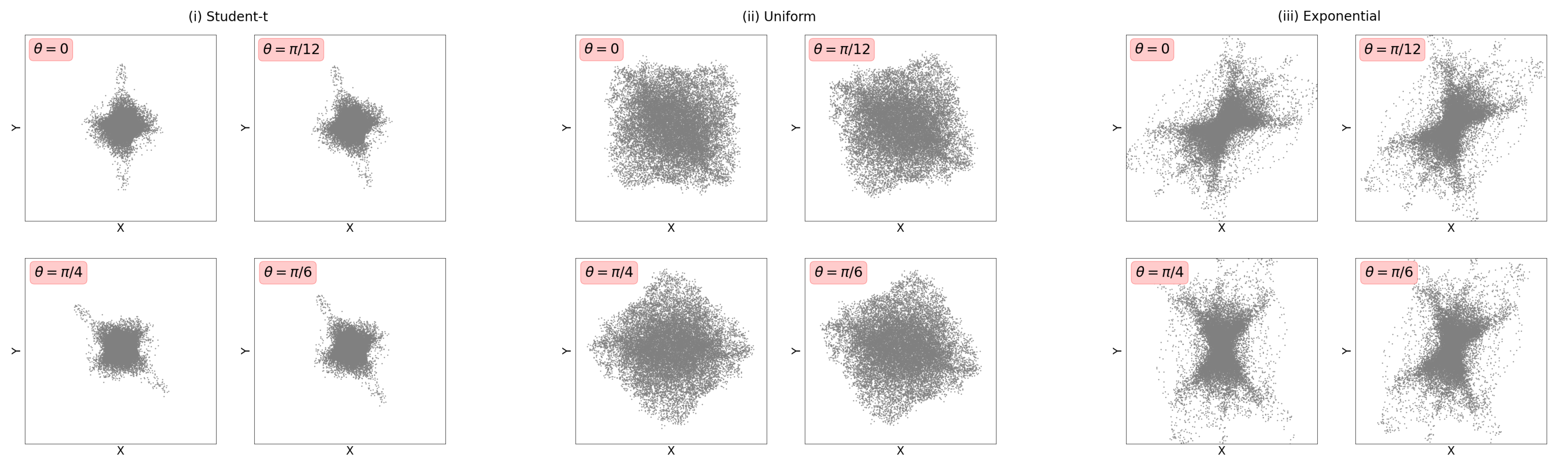
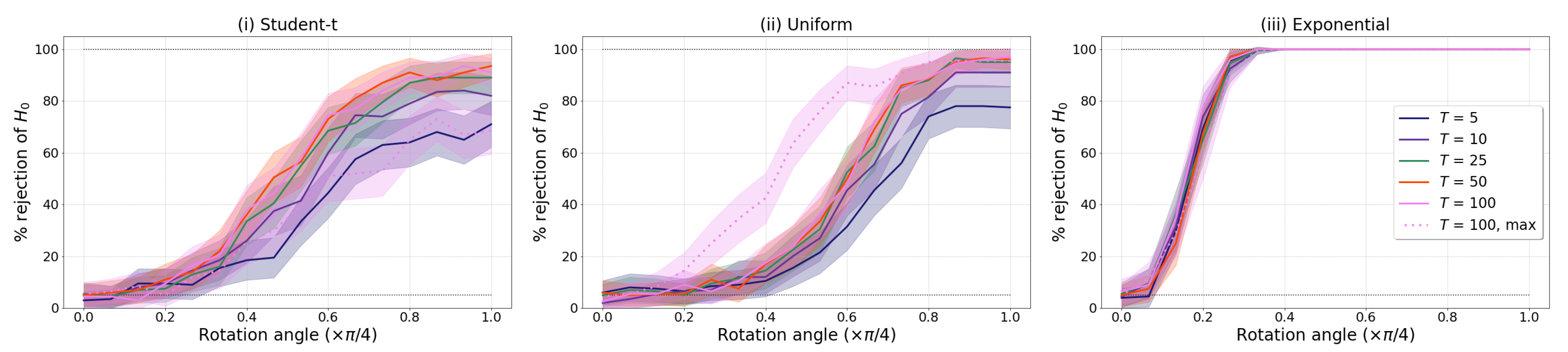
• Dependence through rotation: We start by generating independent ${\mathbf{X}}^{\left(0\right)}$ and ${\mathbf{Y}}^{\left(0\right)}$ as in (9) with ${\mu }_{\mathbf{X}}\left(t\right)={\mu }_{\mathbf{Y}}\left(t\right)=t$ and ${{ϵ}_{\mathbf{X}}}_{i,t},{{ϵ}_{\mathbf{Y}}}_{i,t}\sim \mathcal{N}(0,0.25)$, but with ${{\xi }_{\mathbf{X}}}_{i,k}$ and ${{\xi }_{\mathbf{Y}}}_{i,k}$ drawn from: (i) student-t, (ii) uniform, or (iii) exponential distributions [28] (Table 3). We next multiply $({\mathbf{X}}^{\left(0\right)},{\mathbf{Y}}^{\left(0\right)})$ by a $2\times 2$ rotation matrix $R\left(\theta \right)$ with $\theta \in [0,\pi /4]$ to generate new rotated samples $(\mathbf{X},\mathbf{Y})$, which we then test for independence. Clearly, for $\theta =0$ our samples $(\mathbf{X},\mathbf{Y})$ are independent and as $\theta$ is increased their dependence becomes easier to detect (see [7] (Section 4) and Figure A3 for implementation details).

Statistical significance is computed using $P=5000$ permutations of $\mathbf{Y}$ whilst $\mathbf{X}$ is kept fixed to approximate the distribution under $H_0$. Test power is calculated for varying $T=[5,10,25,50,100]$ and different sample sizes $m=n$.

4.2.2. Baseline Results without Test Power Optimisation

Our baseline results are computed using a Gaussian kernel with $\sigma$ equal to the median distance between measurements in the corresponding sample. Figure 3 (left) shows the results of our test on the linear dependence experiments, which demonstrate, due to $T_{\mathbf{Y}}=1$, how dependencies between individual points in time and an entire time series can be detected. We compare our method to: (i) a statistic explicitly aimed at linear dependence, $\mathrm{SubCorr}=\frac{1}{T_{\mathbf{X}}}{\sum }_{t=1}^{T_{\mathbf{X}}}\mathrm{Corr}({\left\{x_{i,t}\right\}}_{i=1}^m,\mathbf{Y})$, where $\mathrm{Corr}(·,·)$ is the Pearson correlation coefficient; and (ii) $\mathrm{SubHSIC}=\frac{1}{T_{\mathbf{X}}}{\sum }_{t=1}^{T_{\mathbf{X}}}{\widehat{{\displaystyle \mathrm{HSIC}}}}_u({\left\{x_{i,t}\right\}}_{i=1}^m,\mathbf{Y})$. For both of these methods, the distribution under $H_0$ is also approximated via permutations. We find that SubCorr outperforms the other methods in experiments with sample sizes $m<20$, and SubHSIC achieves comparable results to our method. The results for $T_{\mathbf{X}}=[25,50,100]$ (see Appendix A.1) are similar.

Figure 3. Results of the hsic-based independence test: Test power for linear dependence (left) and dependence through shared coefficients (right) as sample size is varied for various numbers of time points. For the linear dependence, we compare our baseline results to SubCorr and SubHSIC; for the shared coefficient, we compare against two spectral approximations [18] (Section 5.1).

Figure 3 (right) displays the power of our independence test for the case of dependent samples through a shared coefficient for varying sample sizes m and measurements T. We compare our results to two spectral methods [18] that approximate the distribution under $H_0$ using eigenvalues of the centred kernel matrices of $\mathbf{X}$ and $\mathbf{Y}$: spectral hsic uses the unbiased estimator (4) as the test statistic with the eigenvalue-based null distribution; and spectral rff uses a test statistic induced by a number of random Fourier feature (rffs) (set here to 10) that approximate the kernel matrices of $\mathbf{X}$ and $\mathbf{Y}$. Our method and spectral hsic achieve $20-50\%$ improvement in test power compared to spectral rff. For small numbers of samples ($m<15$), our method outperforms spectral hsic, which converges to the performance of our method with increasing sample size, as we would expect it [22] (Theorem 1).

Figure 4 shows the rotation dependence experiments, where $\theta =0$ corresponds to the null hypothesis (independence) and $\theta >0$ to the alternative. The distribution hyperparameters for ${{\xi }_{\mathbf{X}}}_{i,k}$ and ${{\xi }_{\mathbf{Y}}}_{i,k}$ are detailed in Appendix A.3, and we set $T_{\mathbf{X}}=T_{\mathbf{Y}}=T$, although equality is not required. As expected, dependence is easier to detect with increasing $\theta$. We observe that denser temporal measurements do not result in enhanced test power. Note that the test power is highly dependent on the distribution of the coefficients of the basis functions ${{\xi }_{\mathbf{X}}}_{i,k}$, ${{\xi }_{\mathbf{Y}}}_{i,k}$.

Figure 4. Results of the hsic-based independence test: Percentage of rejected $H_0$ in rotation dependence experiments for different number of discrete time points T and coefficients ${{\xi }_{\mathbf{X}}}_{i,k}$ and ${{\xi }_{\mathbf{Y}}}_{i,k}$ drawn from three distributions: (i) student-t, (ii) uniform, and (iii) exponential (see Appendix A.3). The sample size is $m=200$. The violet dotted lines are the results of our test power maximisation.

4.2.3. Results of the Optimised Test

The test power maximisation was applied to the rotation dependence experiments by searching for optimal Gaussian kernel bandwidths ${\sigma }_{\mathbf{X}}$ and ${\sigma }_{\mathbf{Y}}$ over predefined intervals (specified in Appendix A.2). Figure 4 shows that the test power is improved when the basis function coefficients are drawn from uniform distributions. In this case, the percentage of rejected $H_0$ is $20-40\%$ higher for $\theta$ between $0.2$ and $0.75\times \pi /4$, but it levels off at $95\%$ once $\theta \ge 0.75\times \pi /4$, which is the same level achieved by our baseline method for $\theta \ge 0.85\times \pi /4$. With our current test-train split, our optimised test does not improve the test power if the basis function coefficients ${{\xi }_{\mathbf{X}}}_{i,k}$ and ${{\xi }_{\mathbf{Y}}}_{i,k}$ are drawn from student-t or exponential distributions.

5. Application to a Socioeconomic Dataset

As a further illustration, we apply our method to the United Nations’ socioeconomic Sustainable Development Goal (sdgs) (see Appendix A.4 for details). Specifically, we investigate whether some so-called Targets of the 17 sdgs have been homogeneous over the last 20 years across low- and high-income countries and whether certain sdgs in African countries exhibit dependence over the same period. In both settings, we assume countries are independent.

For our homogeneity tests, we classify countries into low- and high-income according to [29]. We use temporal data of 76 Targets for which [30] provides data collected over the last $T=20$ years for $m=30$ low-income countries and $n=55$ high-income countries. Applying our baseline method without test power optimisation, we find that, out of the 76 Targets we have data available for, only 38 have had homogeneous trajectories in low- and high-income countries. For instance, whereas the ‘death rate due to road traffic injuries’ (Target 3.6) has been homogeneous between these two groups, the ‘fight the epidemics of AIDS, tuberculosis, malaria and others’ (Target 3.3) has not been homogeneous in low- and high-income countries.

For our independence tests, we consider temporal data from $m=n=49$ African countries over $T=20$ years and test any two Targets for pairwise independence. Of the total 2850 possible pairwise combinations, the null hypothesis of independence is rejected for 357. As an illustration, we examine the dependencies of ‘implementation of national social protection systems’ (Target 1.3) with ‘economic growth’ (Target 8.1) and the ‘proportion of informally employed workers’ (Target 8.3). Applying our baseline method, we accept the null hypothesis of independence between Target 1.3 and 8.1, i.e., we find that the ‘implementation of national social protection systems’ has been independent of economic growth. In contrast, we find that Target 1.3 has been dependent on the ‘proportion of informally employed workers’ (Target 8.3).

6. Discussion and Conclusions

Building on ideas from functional data analysis, we have presented approaches to testing for homogeneity and independence between two nonstationary random processes with the kernel-based statistics mmd and hsic. We view independent realisations of the underlying processes as samples from multivariate probability distributions to which mmd and hsic can be applied. Our tests are shown to outperform current state-of-the-art methods in a range of experiments. Furthermore, we optimise the test power over the choice of kernel and achieve improved results in most settings. However, we also observe that our optimisation procedure does not always yield an increase in test power. We leave the investigation of this behaviour open for future research with the possibility of defining search spaces and step sizes over kernel hyperparameters differently or of choosing a gradient-based approach for optimisation [27]. Our results show that small sample sizes of less than 40 independent realisations can already achieve high test power and that denser measurements over the same time period do not necessarily lead to enhanced test power.

The proposed tests can be of interest in many areas where nonstationary and nonlinear multivariate temporal datasets constitute the norm, as illustrated by our application to test for homogeneity and independence between the United Nations’ Sustainable Development Goals measured in different countries over the last 20 years.

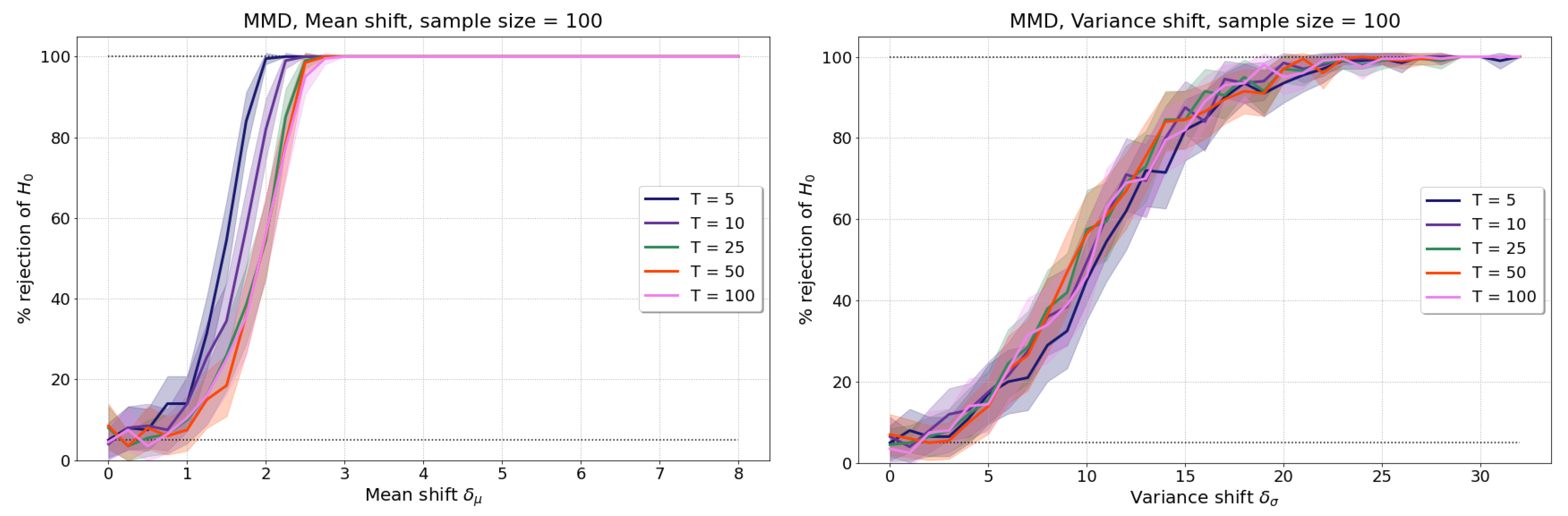
Appendix A.1. Results for Realisations with Varying Number of Time Points, T

mmd We show here the results for mean and variance shifts for $m=n=100$, but the results are similar for all tested sample sizes $m=n=100,200,300,500$,

Figure A1. Results of mmd-based homogeneity test with $T=[5,10,25,50,100]$: Percentage of rejected $H_0$ for mean shift (left) and variance shift (right) for sample sizes $m=n=100$ and T discrete time points in $d=1$ dimensions.

Figure A1. Results of mmd-based homogeneity test with $T=[5,10,25,50,100]$: Percentage of rejected $H_0$ for mean shift (left) and variance shift (right) for sample sizes $m=n=100$ and T discrete time points in $d=1$ dimensions.

hsic Experiments for linear dependence and dependence through shared second basis function coefficient for various T. We find that the granularity of measurements over time does not influence the text power significantly.

Figure A2. Results of the hsic-based independence test: Test power for linear dependence (left) and dependence through shared coefficient (right) as sample size is varied for various numbers of time points $T=[5,10,25,50,100]$.

Figure A2. Results of the hsic-based independence test: Test power for linear dependence (left) and dependence through shared coefficient (right) as sample size is varied for various numbers of time points $T=[5,10,25,50,100]$.

Appendix A.2. Test Power Maximisation

mmd For mean shift experiments for mmd, we predefine a linear search space with 11 values for the Gaussian kernel bandwidth $\sigma$ due to the dependence on ${\delta }_{\mu }$ and similarly for variance shift experiments (both stated in Table A1). These search spaces resulted from extensive manual explorations for all shifts and sample sizes. We acknowledge that the test power may be further improved with search spaces of finer granularity.

hsic We define search intervals of both ${\sigma }_{\mathbf{X}}$ and ${\sigma }_{\mathbf{Y}}$ across all angles $\theta$ but different for the student-t, uniform, and exponential distributions. For student-t and exponential distributions, both ${\sigma }_{\mathbf{X}}$ and ${\sigma }_{\mathbf{Y}}$ were chosen as 20 evenly spaced numbers on a linear scale between 1 and 20. For uniform distributions, both ${\sigma }_{\mathbf{X}}$ and ${\sigma }_{\mathbf{Y}}$ were chosen as 40 evenly spaced numbers on a linear scale between 1 and 40. These search spaces resulted from extensive manual explorations for all angles and distributions. We acknowledge that the test power may be further improved with search spaces of finer granularity.

Table A1. Linear search spaces for bandwidth $\sigma$ in mmd mean (left) and variance (right) shift experiments.

${\mathbf{\delta }}_{\mathbf{\mu }}$	0–2	2.25–3	3.25–5	5.5–8	${\mathbf{\delta }}_{\mathbf{\sigma }}$	0–4	5–14	15–32
	Step Size = 0.25			Step Size = 0.5		Step Size = 1
search space for $\sigma$	1	6	11	16	search space for $\sigma$	10	20	30
	3	8	13	18		12	22	32
	5	10	15	20		14	24	34
	7	12	17	22		16	26	36
	9	14	19	24		18	28	38
	11	16	21	26		20	30	40
	13	18	23	28		22	32	42
	15	20	25	30		24	34	44
	17	22	27	32		26	36	46
	19	24	29	34		28	38	48
	21	26	31	36		30	40	50

Table A1. Linear search spaces for bandwidth $\sigma$ in mmd mean (left) and variance (right) shift experiments.

${\mathbf{\delta }}_{\mathbf{\mu }}$	0–2	2.25–3	3.25–5	5.5–8	${\mathbf{\delta }}_{\mathbf{\sigma }}$	0–4	5–14	15–32
	Step Size = 0.25			Step Size = 0.5		Step Size = 1
search space for $\sigma$	1	6	11	16	search space for $\sigma$	10	20	30
	3	8	13	18		12	22	32
	5	10	15	20		14	24	34
	7	12	17	22		16	26	36
	9	14	19	24		18	28	38
	11	16	21	26		20	30	40
	13	18	23	28		22	32	42
	15	20	25	30		24	34	44
	17	22	27	32		26	36	46
	19	24	29	34		28	38	48
	21	26	31	36		30	40	50

Appendix A.3. Distribution Specifications for Basis Function Coefficients in Rotation Mixing

Table A2. Specifications of distributions for the rotation mixing. They are a subset of the distributions in [28] (Table 3), and $\mathbf{Z}$ is a proxy for both $\mathbf{X}$ and $\mathbf{Y}$.

Distribution	Fourier Basis Function Coefficients
	${\mathbf{\xi }}_{\mathbf{Z}\mathbf{i}\mathbf{1}}$	${\mathbf{\xi }}_{\mathbf{Z}\mathbf{i}\mathbf{2}}$
Exponential	$\lambda =1.5$	$\lambda =3$
Student-t	$\nu =3$	$\nu =5$
Uniform	$\mathcal{U}[-10,10]$	$\mathcal{U}[-5,5]$

Table A2. Specifications of distributions for the rotation mixing. They are a subset of the distributions in [28] (Table 3), and $\mathbf{Z}$ is a proxy for both $\mathbf{X}$ and $\mathbf{Y}$.

Distribution	Fourier Basis Function Coefficients
	${\mathbf{\xi }}_{\mathbf{Z}\mathbf{i}\mathbf{1}}$	${\mathbf{\xi }}_{\mathbf{Z}\mathbf{i}\mathbf{2}}$
Exponential	$\lambda =1.5$	$\lambda =3$
Student-t	$\nu =3$	$\nu =5$
Uniform	$\mathcal{U}[-10,10]$	$\mathcal{U}[-5,5]$

Figure A3. Illustration of $\mathbf{X}$ and $\mathbf{Y}$ with (i) student-t, (ii) uniform, and (iii) exponential basis function coefficients being mixed by different rotation angles $\theta$, ordered clockwise by increasing $\theta$.

Figure A3. Illustration of $\mathbf{X}$ and $\mathbf{Y}$ with (i) student-t, (ii) uniform, and (iii) exponential basis function coefficients being mixed by different rotation angles $\theta$, ordered clockwise by increasing $\theta$.

Appendix A.4. SDG Dataset

Data of the Indicators measuring the progress of the Targets of the sdgs can be found at [30]. Each of these Indicators measures the progress towards a specific Target. For instance, an Indicator for Target 1.1, ‘by 2030, eradicate extreme poverty for all people everywhere, currently measured as people living on less than $1.90 a day’, is the ‘proportion of population below the international poverty line, by gender, age, employment status and geographical location (urban/rural)’. Each of the Targets belongs to one specific Goal (e.g., Target 1.1 belongs to Goal 1, ‘end poverty in all its forms everywhere’). There are 17 such Goals, which are commonly referred to as the Sustainable Development Goals (sdgs). We compute averages over all Indicators belonging to one Target for our analyses in Section 5.

The dataset of [30] has many missing values, especially for the time span 2000–2005. We impute these values using a weighted average across countries (where data is available) with weights inversely proportional to the Euclidean distance between indicators.

References

- Christakis, N.A.; Fowler, J.H. The spread of obesity in a large social network over 32 years. N. Engl. J. Med. 2007, 357, 370–379. [Google Scholar] [CrossRef] [PubMed] [Green Version]
- Barabási, A.L.; Gulbahce, N.; Loscalzo, J. Network medicine: A network-based approach to human disease. Nat. Rev. Genet. 2011, 12, 56–68. [Google Scholar] [CrossRef] [Green Version]
- Bond, R. Complex networks: Network healing after loss. Nat. Hum. Behav. 2017, 1, 1–2. [Google Scholar] [CrossRef]
- Battiston, S.; Mandel, A.; Monasterolo, I.; Schütze, F.; Visentin, G. A climate stress-test of the financial system. Nat. Clim. Chang. 2017, 7, 283–288. [Google Scholar] [CrossRef]
- Muandet, K.; Fukumizu, K.; Sriperumbudur, B.; Schölkopf, B. Kernel mean embedding of distributions: A review and beyond. Found. Trends Mach. Learn. 2017, 10, 1–141. [Google Scholar] [CrossRef]
- Gretton, A.; Borgwardt, K.; Rasch, M.; Schölkopf, B.; Smola, A.J. A kernel method for the two-sample-problem. arXiv 2008, arXiv:0805.2368. [Google Scholar]
- Gretton, A.; Fukumizu, K.; Teo, C.H.; Song, L.; Schölkopf, B.; Smola, A.J. A kernel statistical test of independence. NIPS 2008, 20, 585–592. [Google Scholar]
- Besserve, M.; Logothetis, N.K.; Schölkopf, B. Statistical analysis of coupled time series with Kernel Cross-Spectral Density operators. In Advances in Neural Information Processing Systems 26; Curran Associates, Inc.: Red Hook, NY, USA, 2013; pp. 2535–2543. [Google Scholar]
- Chwialkowski, K.; Sejdinovic, D.; Gretton, A. A wild bootstrap for degenerate kernel tests. In Advances in Neural Information Processing Systems; Curran Associates, Inc.: Red Hook, NY, USA, 2014; pp. 3608–3616. [Google Scholar]
- Davis, R.A.; Matsui, M.; Mikosch, T.; Wan, P. Applications of distance correlation to time series. Bernoulli 2018, 24, 3087–3116. [Google Scholar] [CrossRef] [Green Version]
- Székely, G.J.; Rizzo, M.L.; Bakirov, N.K. Measuring and testing dependence by correlation of distances. Ann. Stat. 2007, 35, 2769–2794. [Google Scholar] [CrossRef]
- Horváth, L.; Kokoszka, P.; Reeder, R. Estimation of the mean of functional time series and a two-sample problem. J. R. Stat. Soc. Ser. B 2012, 75, 103–122. [Google Scholar] [CrossRef] [Green Version]
- Fremdt, S.; Steinbach, J.G.; Horváth, L.; Kokoszka, P. Testing the Equality of Covariance Operators in Functional Samples. Scand. J. Stat. 2012, 40, 138–152. [Google Scholar] [CrossRef] [Green Version]
- Panaretos, V.M.; Kraus, D.; Maddocks, J.H. Second-Order Comparison of Gaussian Random Functions and the Geometry of DNA Minicircles. J. Am. Stat. Assoc. 2010, 105, 670–682. [Google Scholar] [CrossRef] [Green Version]
- Pomann, G.M.; Staicu, A.M.; Ghosh, S. A two-sample distribution-free test for functional data with application to a diffusion tensor imaging study of multiple sclerosis. J. R. Stat. Soc. Ser. C 2016, 65, 395–414. [Google Scholar] [CrossRef] [PubMed] [Green Version]
- Wynne, G.; Duncan, A.B. A kernel two-sample test for functional data. arXiv 2020, arXiv:2008.11095. [Google Scholar]
- Górecki, T.; Krzyśko, M.; Wołyński, W. Independence test and canonical correlation analysis based on the alignment between kernel matrices for multivariate functional data. Artif. Intell. Rev. 2018, 53, 475–499. [Google Scholar] [CrossRef] [Green Version]
- Zhang, Q.; Filippi, S.; Gretton, A.; Sejdinovic, D. Large-scale kernel methods for independence testing. Stat. Comput. 2018, 28, 113–130. [Google Scholar] [CrossRef] [Green Version]
- Sriperumbudur, B.K.; Gretton, A.; Fukumizu, K.; Schölkopf, B.; Lanckriet, G.R. Hilbert space embeddings and metrics on probability measures. J. Mach. Learn. Res. 2010, 11, 1517–1561. [Google Scholar]
- Sriperumbudur, B.K.; Fukumizu, K.; Lanckriet, G.R. Universality, Characteristic Kernels and RKHS Embedding of Measures. J. Mach. Learn. Res. 2011, 12, 2389–2410. [Google Scholar]
- Gretton, A.; Borgwardt, K.M.; Rasch, M.J.; Schölkopf, B.; Smola, A.J. A kernel two-sample test. J. Mach. Learn. Res. 2012, 13, 723–773. [Google Scholar]
- Gretton, A.; Fukumizu, K.; Harchaoui, Z.; Sriperumbudur, B.K. A fast, consistent kernel two-sample test. NIPS 2009, 23, 673–681. [Google Scholar]
- Song, L.; Smola, A.J.; Gretton, A.; Bedo, J.; Borgwardt, K. Feature selection via dependence maximization. J. Mach. Learn. Res. 2012, 13, 1393–1434. [Google Scholar]
- Ramdas, A.; Reddi, S.J.; Póczos, B.; Singh, A.; Wasserman, L. On the decreasing power of kernel and distance based nonparametric hypothesis tests in high dimensions. In Proceedings of the Twenty-Ninth AAAI Conference on Artificial Intelligence, Austin, TX, USA, 25–30 January 2015. [Google Scholar]
- Reddi, S.; Ramdas, A.; Póczos, B.; Singh, A.; Wasserman, L. On the high dimensional power of a linear-time two sample test under mean-shift alternatives. Artif. Intell. Stat. 2015, 38, 772–780. [Google Scholar]
- Serfling, R.J. Approximation Theorems of Mathematical Statistics; Wiley Series in Probability and Mathematical Statistics; Wiley: New York, NY, USA, 2002. [Google Scholar]
- Sutherland, D.J.; Tung, H.Y.; Strathmann, H.; De, S.; Ramdas, A.; Smola, A.J.; Gretton, A. Generative models and model criticism via optimized maximum mean discrepancy. arXiv 2016, arXiv:1611.04488. [Google Scholar]
- Gretton, A.; Herbrich, R.; Smola, A.J.; Bousquet, O.; Schölkopf, B. Kernel methods for measuring independence. J. Mach. Learn. Res. 2005, 6, 2075–2129. [Google Scholar]
- World Bank. World Bank Country and Lending Groups. 2020. Available online: https://datahelpdesk.worldbank.org/knowledgebase/articles/906519-world-bank-country-and-lending-groups (accessed on 28 January 2020).
- World Bank. Sustainable Development Goals. 2020. Available online: https://datacatalog.worldbank.org/dataset/sustainable-development-goals (accessed on 28 January 2020).
Publisher’s Note: MDPI stays neutral with regard to jurisdictional claims in published maps and institutional affiliations. |
© 2021 by the authors. Licensee MDPI, Basel, Switzerland. This article is an open access article distributed under the terms and conditions of the Creative Commons Attribution (CC BY) license (https://creativecommons.org/licenses/by/4.0/).