
Meta-Parameter Selection for Embedding Generation of Latency Spaces in Auto Encoder Analytics †


Abstract
:1. Introduction
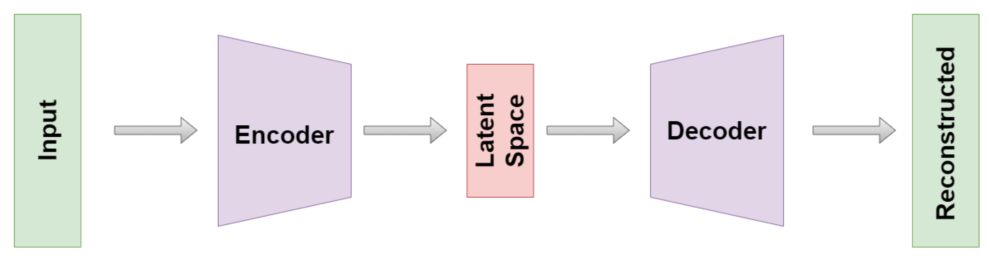
1.1. Why Are Autoencoders Interesting?
1.2. Our Approach
1.3. Embedding and Visualization Methods
1.3.1. t-SNE
1.3.2. UMAP
1.3.3. k-MEANS
1.3.4. DBSCAN
1.3.5. OPTICS
1.4. Organization and Contribution of the Paper
- autoencoder study on DeepVALVE data set
- cross-correlative study of embedding technologies
- procedure to gain manageable meta-parameter ranges
- visual analysis of autoencoder latency spaces
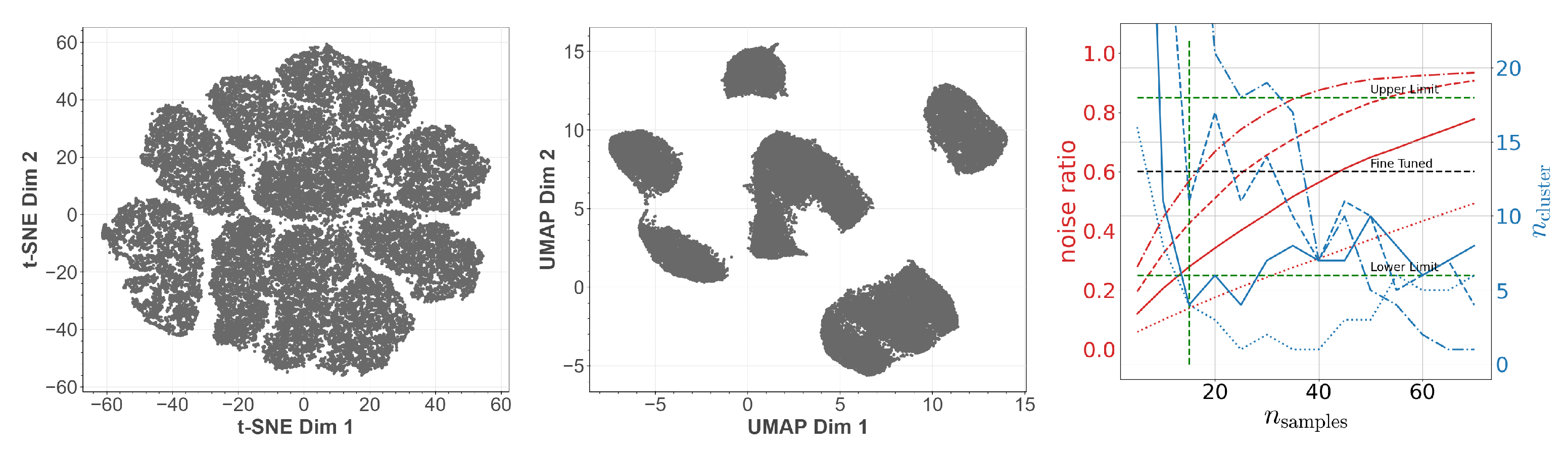
2. Cross-Correlative Study on Meta-Parameters
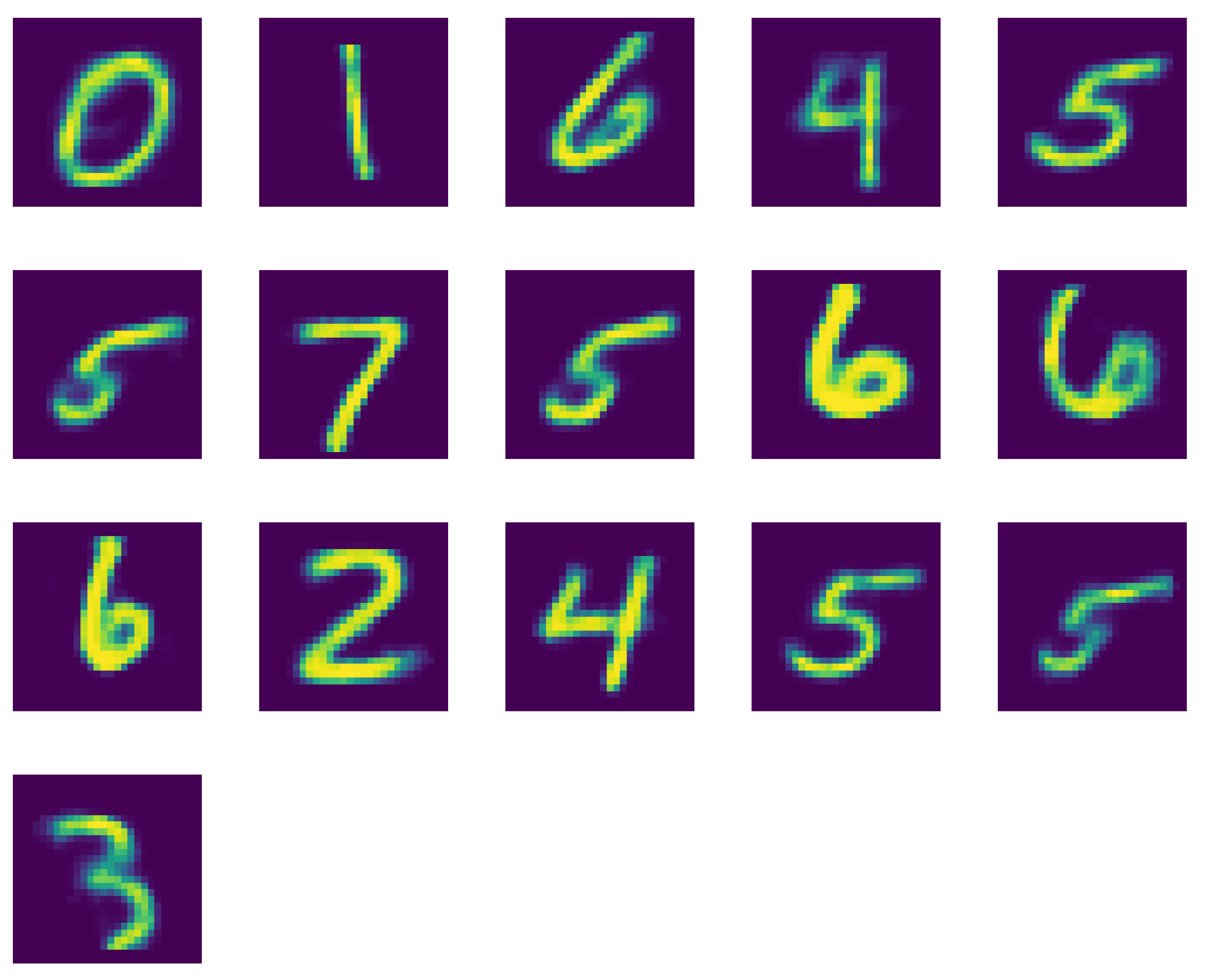
2.1. MNIST
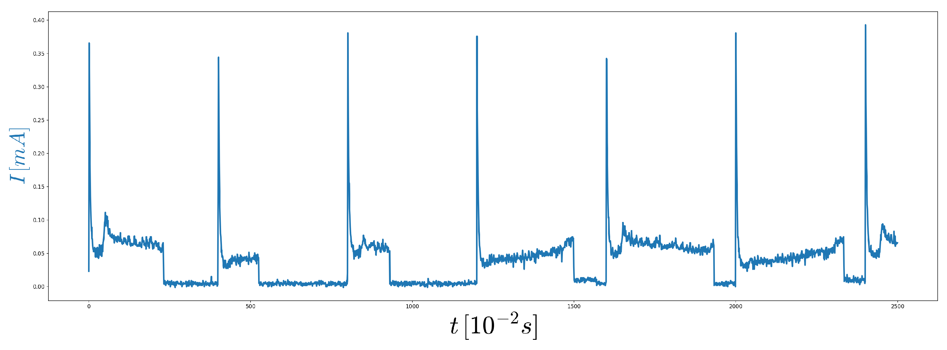
2.2. DeepVALVE
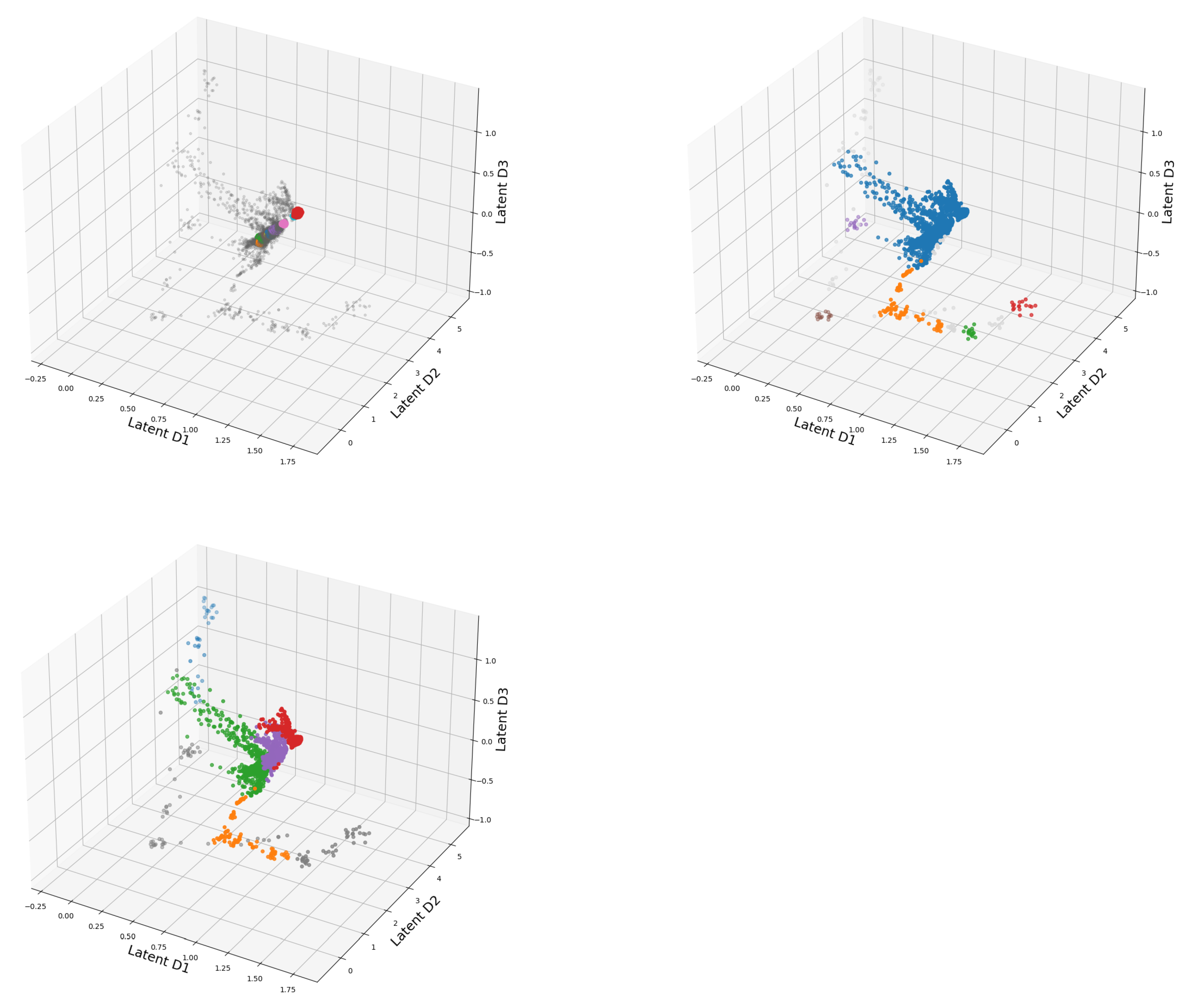
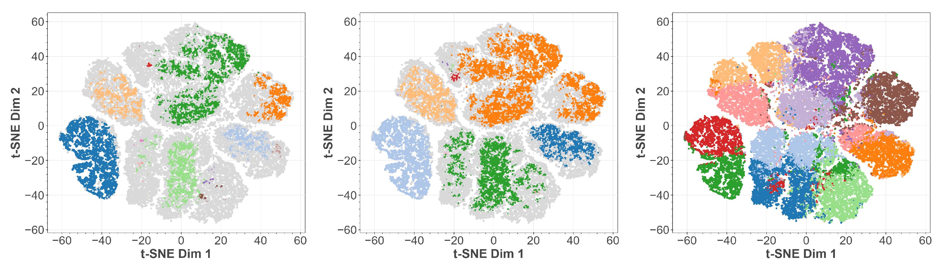
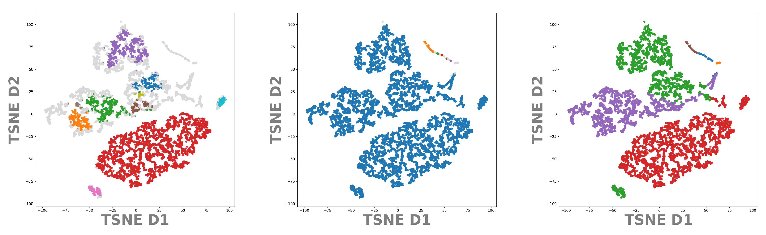
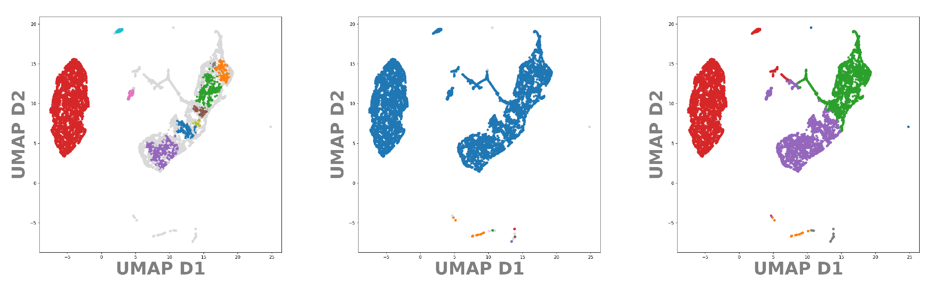
3. Visualization of Clustered Data
4. Conclusions
- (i)
- We developed a pipeline to obtain a visual grasp on the generalization capacity of a vanilla autoencoder.
- (ii)
- We use clustering and embedding methods in a cross-correlative way to fine-tune their observational capabilities.
- (iii)
- This cross-correlative ansatz allows better capture of the interrelation between the (transformed) data and the visualizations and embeddings.
- (iv)
- Doing so, structural differences between data sets become apparent, which allows obtaining a first apprehension of an unknown data set without prior knowledge.
4.1. The Generalization Capacity vs. the Manifold Hypothesis
4.2. Meta-Parameter Fine-Tuning
4.3. Interrelation between Data and Methodology
4.4. Structural Differences between Data Sets
4.5. Future Outlook and Comparison to Other Work
Data Availability Statement
Appendix A. Autoencoder Hyperparameters and Architecture for Reproducibility

| Hyperparameter | Values |
|---|---|
| Learning Rate | |
| Optimizer | Adam |
| Random Seed | 0 |
| Activation Function of hidden layers | ReLU |
| Activation Function of output layer | Sigmoid |
| Epochs | 100 |
| Batch Size | 100 |
| Loss | Mean Square Error |
| Data Set | Input Size | Architecture | |
|---|---|---|---|
| MNIST | 784 | ||
| DeepVALVE | 10 |
Appendix B. Meta-Parameter Default Values
| Embedding Method | Meta-Parameters Used and Their Default Values |
|---|---|
| t-SNE | , |
| UMAP | , |
| DBSCAN | , |
| OPTICS | , |
| K-Means | , , |
| , , , | |
Appendix C. Additional Material for MNIST
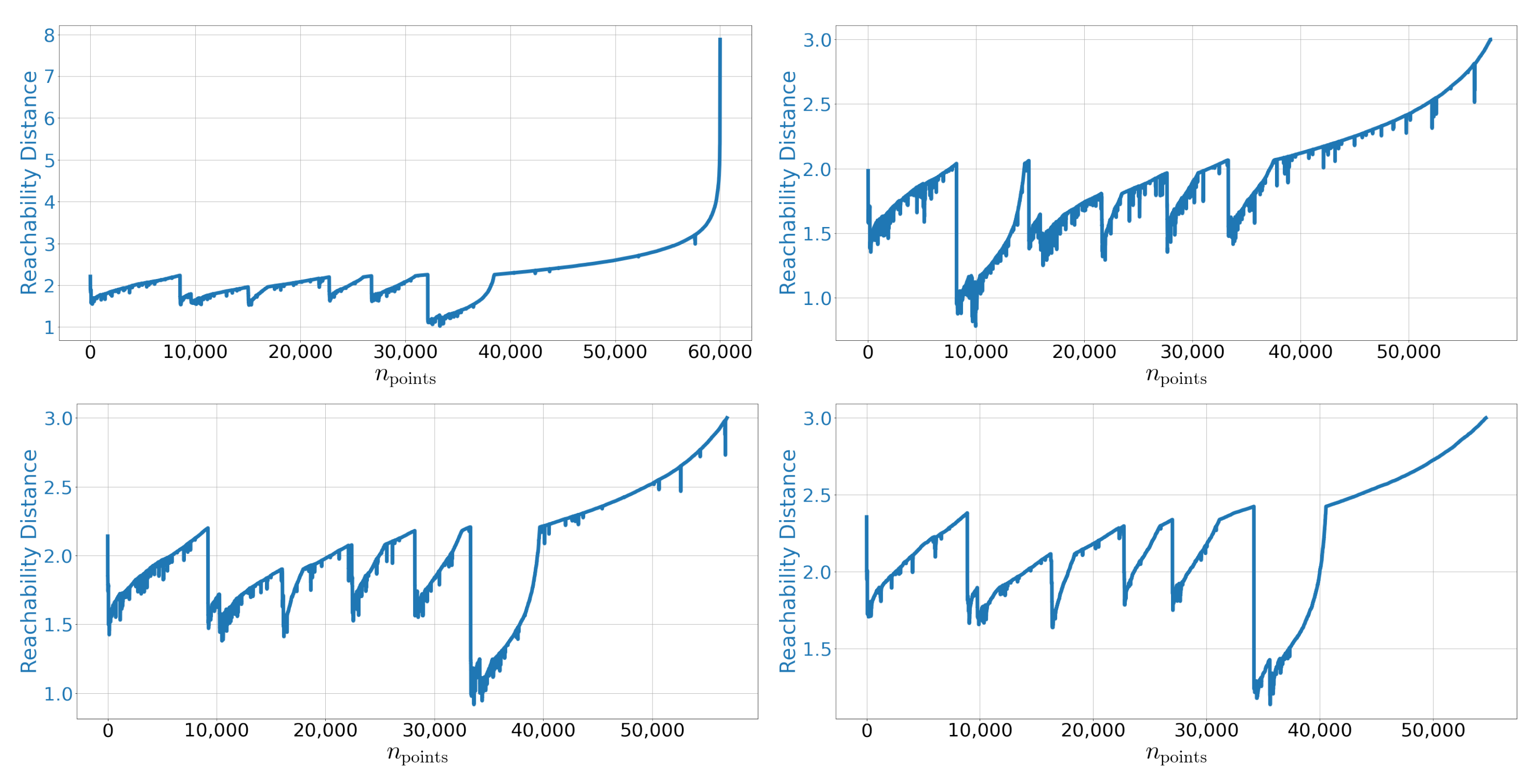
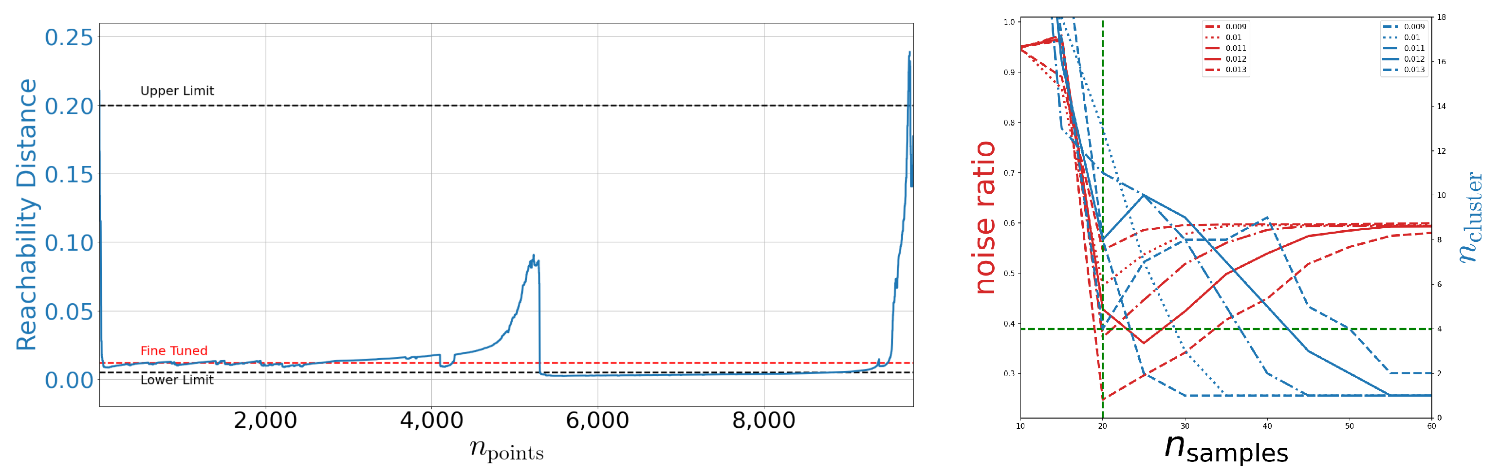
Appendix C.1. Reachability Plots

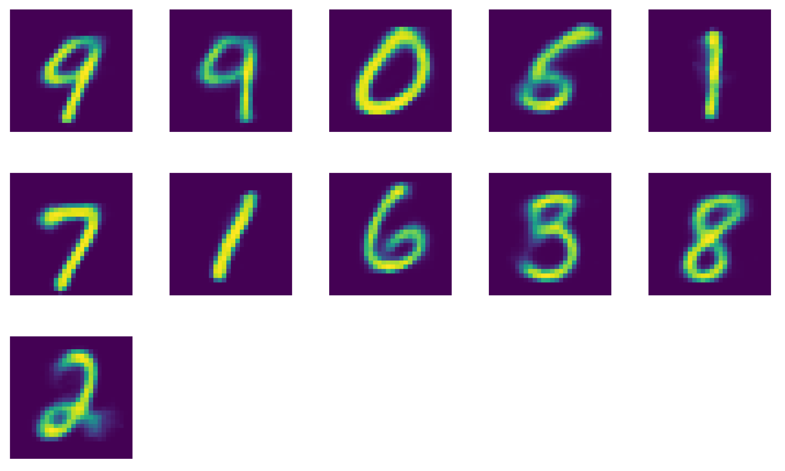
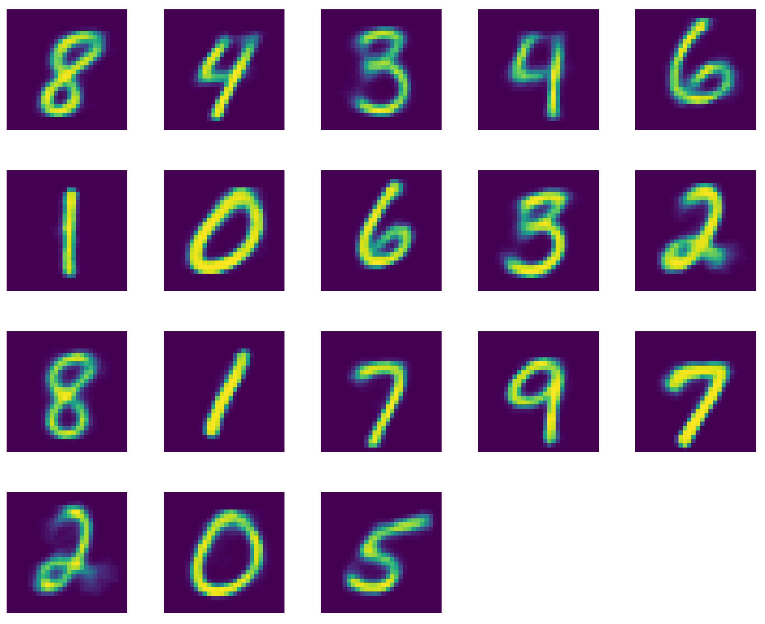
Appendix C.2. Reconstructed Digits


Appendix D. Additional Material for DeepVALVE

References
- Donoho, D.L. High-dimensional data analysis: The curses and blessings of dimensionality. In Proceedings of the AMS Conference on Math Challenges of the 21st Century, Los Angeles, CA, USA, 7–12 August 2000. [Google Scholar]
- Sembiring, R.W.; Mohamad Zain, J.; Abdullah, E. Dimension Reduction of Health Data Clustering. arXiv 2011, arXiv:1110.3569. [Google Scholar]
- Chen, Y.; Tang, S.; Bouguila, N.; Wang, C.; Du, J.; Li, H. A Fast Clustering Algorithm based on pruning unnecessary distance computations in DBSCAN for High-Dimensional Data. Pattern Recognit. 2018, 83. [Google Scholar] [CrossRef]
- Deng, L. The mnist database of handwritten digit images for machine learning research. IEEE Signal Process. Mag. 2012, 29, 141–142. [Google Scholar] [CrossRef]
- Ahmed, S.; Schichtel, P.; von der Ohe, T. Sensorlose Prozesse mit kuenstlicher Intelligenz erfassen und steuern. MTZextra 2018, 23, 42–45. [Google Scholar] [CrossRef]
- Rumelhart, D.; Hinton, G.; Williams, R. Parallel Distributed Processing. Volume 1: Foundations; MIT Press: Cambridge, UK, 1986. [Google Scholar]
- Bank, D.; Koenigstein, N.; Giryes, R. Autoencoders. arXiv 2021, arXiv:2003.05991. [Google Scholar]
- Rossler, A.; Cozzolino, D.; Verdoliva, L.; Riess, C.; Thies, J.; Niessner, M. FaceForensics++: Learning to Detect Manipulated Facial Images. In Proceedings of the IEEE/CVF International Conference on Computer Vision (ICCV), Seoul, Korea, 27 October–2 November 2019. [Google Scholar]
- Zhang, Y.; Lee, K.; Lee, H. Augmenting Supervised Neural Networks with Unsupervised Objectives for Large-scale Image Classification. In Proceedings of the 33rd International Conference on Machine Learning, New York, NY, USA, 19–24 June 2016; Balcan, M.F., Weinberger, K.Q., Eds.; PMLR: New York, NY, USA, 2016; Volume 48, pp. 612–621. [Google Scholar]
- Zhang, B.; Qian, J. Autoencoder-based unsupervised clustering and hashing. Appl. Intell. 2021, 51, 493–505. [Google Scholar] [CrossRef]
- Li, X.; Zhang, T.; Zhao, X.; Yi, Z. Guided autoencoder for dimensionality reduction of pedestrian features. Appl. Intell. 2020, 50, 4557–4567. [Google Scholar] [CrossRef]
- Ferreira, D.; Silva, S.; Abelha, A.; Machado, J. Recommendation System Using Autoencoders. Appl. Sci. 2020, 10, 5510. [Google Scholar] [CrossRef]
- Takeishi, N.; Kalousis, A. Physics-Integrated Variational Autoencoders for Robust and Interpretable Generative Modeling. arXiv 2021, arXiv:2102.13156. [Google Scholar]
- Goodfellow, I.; Bengio, Y.; Courville, A. Deep Learning; MIT Press: Cambridge, MA, USA, 2016; Available online: http://www.deeplearningbook.org (accessed on 7 May 2021).
- Lee, W.; Ortiz, J.; Ko, B.; Lee, R.B. Time Series Segmentation through Automatic Feature Learning. arXiv 2018, arXiv:1801.05394. [Google Scholar]
- Dunteman, G.H. Principal Component Analysis; SAGE Publications: Thousand Oaks, CA, USA, 1989. [Google Scholar]
- Fefferman, C.; Mitter, S.; Narayanan, H. Testing the Manifold Hypothesis. arXiv 2013, arXiv:1310.0425v2. [Google Scholar] [CrossRef]
- Ryck, T.D.; Vos, M.D.; Bertrand, A. Change Point Detection in Time Series Data using Autoencoders with a Time-Invariant Representation. arXiv 2021, arXiv:2008.09524. [Google Scholar]
- Lapuschkin, S.; Wäldchen, S.; Binder, A.; Montavon, G.; Samek, W.; Müller, K.R. Unmasking Clever Hans Predictors and Assessing What Machines Really Learn. Nat. Commun. 2019, 10. [Google Scholar] [CrossRef] [Green Version]
- Moor, M.; Horn, M.; Rieck, B.; Borgwardt, K.M. Topological Autoencoders. arXiv 2019, arXiv:1906.00722. [Google Scholar]
- Pihlgren, G.G.; Sandin, F.; Liwicki, M. Improving Image Autoencoder Embeddings with Perceptual Loss. arXiv 2020, arXiv:2001.03444. [Google Scholar]
- Zhu, Q.; Zhang, R. A Classification Supervised Auto-Encoder Based on Predefined Evenly-Distributed Class Centroids. arXiv 2020, arXiv:1902.00220. [Google Scholar]
- Chel, S.; Gare, S.; Giri, L. Detection of Specific Templates in Calcium Spiking in HeLa Cells Using Hierarchical DBSCAN: Clustering and Visualization of CellDrug Interaction at Multiple Doses. In Proceedings of the 2020 42nd Annual International Conference of the IEEE Engineering in Medicine Biology Society (EMBC), Montreal, QC, Canada, 20–24 July 2020; pp. 2425–2428. [Google Scholar] [CrossRef]
- Cai, T.T.; Ma, R. Theoretical Foundations of t-SNE for Visualizing High-Dimensional Clustered Data. arXiv 2021, arXiv:2105.07536. [Google Scholar]
- Swetha, S.; Kuehne, H.; Rawat, Y.S.; Shah, M. Unsupervised Discriminative Embedding for Sub-Action Learning in Complex Activities. arXiv 2021, arXiv:2105.00067. [Google Scholar]
- Lehmann, D.J.; Theisel, H. Orthographic Star Coordinates. IEEE Trans. Vis. Comput. Graph. 2013, 19, 2615–2624. [Google Scholar] [CrossRef] [Green Version]
- Sánchez, A.; Soguero-Ruiz, C.; Mora-Jimenez, I.; Rivas-Flores, F.J.; Lehmann, D.J.; Rubio-Sánchez, M. Scaled radial axes for interactive visual feature selection: A case study for analyzing chronic conditions. Expert Syst. Appl. 2018, 100, 182–196. Available online: https://www.sciencedirect.com/science/article/pii/S0957417418300617 (accessed on 12 May 2021). [CrossRef]
- Rubio-Sánchez, M.; Sanchez, A.; Lehmann, D.J. Adaptable Radial Axes Plots for Improved Multivariate Data Visualization. Comput. Graph. Forum 2017, 36, 389–399. [Google Scholar] [CrossRef]
- Shao, L.; Mahajan, A.; Schreck, T.; Lehmann, D.J. Interactive Regression Lens for Exploring Scatter Plots. Comput. Graph. Forum 2017, 36, 157–166. [Google Scholar] [CrossRef]
- Wang, Y.; Li, J.; Nie, F.; Theisel, H.; Gong, M.; Lehmann, D.J. Linear Discriminative Star Coordinates for Exploring Class and Cluster Separation of High Dimensional Data. Comput. Graph. Forum 2017, 36, 401–410. [Google Scholar] [CrossRef]
- Lehmann, D.J.; Theisel, H. The LloydRelaxer: An Approach to Minimize Scaling Effects for Multivariate Projections. IEEE Trans. Vis. Comput. Graph. 2017. [Google Scholar] [CrossRef]
- Lehmann, D.J.; Theisel, H. General Projective Maps for Multidimensional Data Projection. Comput. Graph. Forum 2016, 35, 443–453. [Google Scholar] [CrossRef]
- Lehmann, D.J.; Theisel, H. Optimal Sets of Projections of High-Dimensional Data. IEEE Trans. Vis. Comput. Graph. 2015. [Google Scholar] [CrossRef]
- Karer, B.; Hagen, H.; Lehmann, D. Insight Beyond Numbers: The Impact of Qualitative Factors on Visual Data Analysis. IEEE Trans. Vis. Comput. Graph. 2020. [Google Scholar] [CrossRef]
- Rubio-Sánchez, M.; Lehmann, D.; Sanchez, A.; Rojo Álvarez, J. Optimal Axes for Data Value Estimation in Star Coordinates and Radial Axes Plots. Comput. Graph. Forum 2021, 40. [Google Scholar] [CrossRef]
- Pezzotti, N.; Lelieveldt, B.; van der Maaten, L.; Höllt, T.; Eisemann, E.; Vilanova, A. Approximated and User Steerable tSNE for Progressive Visual Analytics. IEEE Trans. Vis. Comput. Graph. 2016, 23, 1739–1752. [Google Scholar] [CrossRef] [PubMed] [Green Version]
- Hinton, G.; Roweis, S. Stochastic Neighbor Embedding. Neural Inf. Process. Syst. 2002, 857–864. [Google Scholar]
- McInnes, L.; Healy, J.; Melville, J. UMAP: Uniform Manifold Approximation and Projection for Dimension Reduction. arXiv 2020, arXiv:1802.03426. [Google Scholar]
- MacQueen, J. Some Methods for Classification and Analysis of Multivariate Observations. Proc. Berkeley Symp. Math. Stat. Probab. 1967, 1, 281–297. [Google Scholar]
- Ester, M.; Kriegel, H.P.; Sander, J.; Xu, X. A Density-Based Algorithm for Discovering Clusters in Large Spatial Databases with Noise; Simoudis, E., Han, J., Fayyad, U.M., Eds.; KDD; AAAI Press: Palo Alto, CA, USA, 1996; pp. 226–231. [Google Scholar]
- Ankerst, M.; Breunig, M.M.; peter Kriegel, H.; Sander, J. OPTICS: Ordering Points To Identify the Clustering Structure; ACM Press: New York, NY, USA, 1999; pp. 49–60. [Google Scholar]
- Hoffman, P.; Grinstein, G.; Marx, K.; Grosse, I.; Stanley, E. DNA visual and analytic data mining. In Proceedings of the Visualization ’97 (Cat. No. 97CB36155), Phoenix, AZ, USA, 19–24 October 1997; pp. 437–441. [Google Scholar] [CrossRef]
- Shamsuddin, M.R.; Rahman, S.; Mohamed, A. Exploratory Analysis of MNIST Handwritten Digit for Machine Learning Modelling. In Proceedings of the 4th International Conference on Soft Computing in Data Science, SCDS 2018, Bangkok, Thailand, 15–16 August 2018; Springer: Singapore, 2019; pp. 134–145. [Google Scholar] [CrossRef]
- Schott, L.; Rauber, J.; Brendel, W.; Bethge, M. Robust Perception through Analysis by Synthesis. arXiv 2018, arXiv:1805.09190. [Google Scholar]
- Tralie, C.J.; Perea, J.A. (Quasi)Periodicity Quantification in Video Data, Using Topology. arXiv 2017, arXiv:1704.08382. [Google Scholar] [CrossRef] [Green Version]
- Ali, M.; Jones, M.W.; Xie, X. TimeCluster: Dimension reduction applied to temporal data for visual analytics. Vis. Comput. 2019, 35, 1013–1026. [Google Scholar] [CrossRef] [Green Version]
- Ali, M.; Alqahtani, A.; Jones, M.W.; Xie, X. Clustering and Classification for Time Series Data in Visual Analytics: A Survey. IEEE Access 2019, 7, 181314–181338. [Google Scholar] [CrossRef]
- Rauber, P.E.; Falcão, A.X.; Telea, A.C. Visualizing Time-Dependent Data Using Dynamic t-SNE; Bertini, E., Elmqvist, N., Wischgoll, T., Eds.; EuroVis 2016—Short Papers; The Eurographics Association: Aire-la-Ville, Switzerland, 2016. [Google Scholar] [CrossRef]
- Vernier, E.F.; Garcia, R.; da Silva, I.P.; Comba, J.L.D.; Telea, A.C. Quantitative Evaluation of Time-Dependent Multidimensional Projection Techniques. arXiv 2020, arXiv:2002.07481. [Google Scholar] [CrossRef]


Publisher’s Note: MDPI stays neutral with regard to jurisdictional claims in published maps and institutional affiliations. |
© 2021 by the authors. Licensee MDPI, Basel, Switzerland. This article is an open access article distributed under the terms and conditions of the Creative Commons Attribution (CC BY) license (https://creativecommons.org/licenses/by/4.0/).
Share and Cite
Walch, M.; Schichtel, P.; Lehmann, D.; Paulson, A. Meta-Parameter Selection for Embedding Generation of Latency Spaces in Auto Encoder Analytics . Eng. Proc. 2021, 5, 30. https://doi.org/10.3390/engproc2021005030
Walch M, Schichtel P, Lehmann D, Paulson A. Meta-Parameter Selection for Embedding Generation of Latency Spaces in Auto Encoder Analytics . Engineering Proceedings. 2021; 5(1):30. https://doi.org/10.3390/engproc2021005030
Chicago/Turabian StyleWalch, Maria, Peter Schichtel, Dirk Lehmann, and Amala Paulson. 2021. "Meta-Parameter Selection for Embedding Generation of Latency Spaces in Auto Encoder Analytics " Engineering Proceedings 5, no. 1: 30. https://doi.org/10.3390/engproc2021005030
APA StyleWalch, M., Schichtel, P., Lehmann, D., & Paulson, A. (2021). Meta-Parameter Selection for Embedding Generation of Latency Spaces in Auto Encoder Analytics . Engineering Proceedings, 5(1), 30. https://doi.org/10.3390/engproc2021005030