Rényi Transfer Entropy Estimators for Financial Time Series  ^†

Abstract

In this paper, we discuss the statistical coherence between financial time series in terms of Rényi’s information measure or entropy. In particular, we tackle the issue of the directional information flow between bivariate time series in terms of Rényi’s transfer entropy. The latter represents a measure of information that is transferred only between certain parts of underlying distributions. This fact is particularly relevant in financial time series, where the knowledge of “black swan” events such as spikes or sudden jumps is of key importance. To put some flesh on the bare bones, we illustrate the essential features of Rényi’s information flow on two coupled GARCH($1,1$) processes.

1. Introduction

The linear framework for measuring and testing causality has been widely applied in a number of fields. In finance, one typically uses Granger’s linear regression model to study the internal cross-correlations between various market activities. The correlation functions have, however, at least two limitations. First, they measure only linear relations, although it is clear that linear models do not faithfully reflect real market interactions. Second, all they determine is whether two time series (e.g., two stock-index series) have correlated movement. They, however, do not indicate which series affects which, or in other words, they do not provide any directional information about cause and effect. However, there is extensive literature on causality modeling that goes beyond the linear regression model, e.g., applying and combining mathematical logic, graph theory, Markov models, Bayesian probability, etc. (for an extensive review see, e.g., [1]). We will focus here on the information-theoretic approaches, which understand causality as a phenomenon that can be not only detected or measured but also quantified. A particularly important quantifier of the information flow between two time series is the so-called transfer entropy (TE).

In his 2000 seminal paper, Schreiber [2] used Shannon’s information measure to formulate the concept of TE, which is a version of mutual information operating on conditional probabilities. TE is designed to detect the directed exchange of information between two stochastic variables, conditioned to common history and inputs. An advantage of information-theoretic measures, in comparison with, say, the standard Granger causality, is that they are sensitive to nonlinear signal properties, as they do not rely on linear regression models. A limitation of TEs is that they are, by their very formulation, restricted to bivariate situations. In addition, information-theoretic measures often require substantially more data than regression methods. It can be also shown that for Gaussian variables, Granger causality and transfer entropy are entirely equivalent [3]. For a comparison of TEs with other causal measures, including various implementations of the Granger causality, see, e.g., Ref. [4].

Shannonian TE was generalized to the class of $\alpha$-Rényi transfer entropies by Jizba et al. in Ref. [5]. The corresponding Rényi TE can be defined in much the same way as its Shannonian counterpart. In particular, one can utilize the concept of mutual information of the order $\alpha$ to quantify the directed exchange of information. Because Rényi’s entropy (RE) works, unlike Shannon’s entropy, with rescaled distributions, it allows addressing information flow between different parts of underlying distributions in bivariate time series. Consequently, Rényi’s TE provides more detailed information concerning the excess (or lack) of information in various parts of the underlying distribution resulting from updating the distribution on the condition that a second time series is known. This is particularly relevant in the context of financial time series, where the knowledge of tale-part (or “black swan”) events such as spikes or sudden jumps bears direct implications, e.g., in various risk-reducing formulas in portfolio theory.

In order to quantify the strength of Rényian information flow and its directionality from high-quality time series data, special care has to be taken to select suitable estimators of Rényi’s entropy. The aim of this paper is to demonstrate that the estimator introduced by Leonenko et al. [6] is an appropriate instrument for this task. We illustrate this by analyzing Rényi’s information flow between two coupled GARCH(1,1) processes.

The paper is organized in the following way. In Section 2, we discuss some essentials from Rényi’s entropy and the ensuing Rényi transfer entropy. Section 3 introduces the concept of effective transfer entropy and briefly discusses the pros and cons of Leonenko et al.’s Rényi entropy estimator. In Section 4, we set up our model system, namely a system of two coupled GARCH processes, that will serve as generating processes for bivariate time series to be analyzed. Section 5 is dedicated to the analysis of the effective Rényi’s TE for coupled GARCH($1,1$) processes. Finally, in Section 6, we provide some concluding remarks and propose some further generalizations.

2. Rényi Transfer Entropy

In this section, we briefly review some essentials of Rényi’s entropy and ensuing directional information flow that will be needed in following sections.

2.1. Rényi Entropy

Rényi’s information measure (also known as Rényi’s entropy) was introduced by Rényi in his seminal 1961 paper [7] as a one-parameter generalization of Shannon’s entropy. Let $\alpha \ge 0$, then Rényi’s entropy of a probability distribution function $\mathcal{P}$ associated with a discrete random variable X is defined as

$$H_{\alpha }\left[\mathcal{P}\right]=\frac{1}{1-\alpha }{log}_2\sum _{x\in X}{p}^{\alpha }\left(x\right).$$

(1)

In particular, for $\alpha =0$, we obtain the so-called Hartley entropy, while the cases with $\alpha =2$ and $\alpha =+\infty$ yield the collision entropy (that is closely related to correlation dimension) and the Min-entropy, respectively. Note that for $\alpha =1$, Rényi’s entropy converges to Shannon’s entropy by the L’Hospital rule. It can be shown [8] that Rényi’s entropy is a non-negative, monotonically decreasing function of $\alpha$, thus

$$H_0\ge H_1\ge H_2\ge H_{+\infty }\ge 0.$$

(2)

Particularly important in our following considerations will be the so-called conditional Rényi entropy that is defined as [8,9]

$$\begin{array}{ccc}\hfill H_{\alpha }\left[\mathcal{P}\right|\mathcal{Q}]& =& \frac{1}{1-\alpha }{log}_2\frac{{\sum }_{x\in X,y\in Y}{p}^{\alpha }(x,y)}{{\sum }_{y\in Y}{p}^{\alpha }\left(y\right)}\hfill \\ & \equiv & \frac{1}{1-\alpha }{log}_2\sum _{y\in Y}{\rho }_{\alpha }\left(y\right)\sum _{x\in X}{p}^{\alpha }\left(x\right|y),\hfill \end{array}$$

(3)

where $\mathcal{Q}$ is a probability distribution function of a random variable Y, and ${\rho }_{\alpha }$, defined as

$${\rho }_{\alpha }\left(x\right)=\frac{p^{\alpha }\left(x\right)}{{\sum }_{x\in X}{p}^{\alpha }\left(x\right)},$$

(4)

is known as escort distribution [10]. The latter is also termed as a “zooming” distribution because it scales (deforms and re-emphasizes) different parts of an underlying distribution function $\mathcal{P}$. In particular, for $\alpha <1$, the central part of the distribution is flattened, i.e., high-probability events are suppressed, and low-probability events are emphasized. This effect is more pronounced for smaller $\alpha$. In the opposite situation when $\alpha >1$, low-probability events are suppressed, and high-probability events are emphasized. Thus, for $\alpha \to 0$, the escort distribution tends to a uniform-like shape and $\alpha \to +\infty$ to a very platykurtic (Dirac’s-$\delta$ function like) distribution. Because this behavior is also true for the conditional RE, it will be seen that REs are instrumental in the understanding of (directional) information flow between bivariate time series.

2.2. Shannon’s and Rényi’s Transfer Entropies

The concept of transfer entropy was introduced by Schreiber in Ref. [2] and independently under the name conditional mutual information by Paluš in Ref. [11]. According to these, TE represents a measure of a directional (Shannonian) information flow defined by means of Kullback–Leibler divergence on conditional transition probabilities of two Markov processes X and Y as

$$T_{X\to Y}(k,l)=\sum _{x\in X,y\in Y}p(y_{n+1},y_n^{\left(l\right)},x_n^{\left(k\right)}){log}_2\frac{p\left(y_{n+1}\right|y_n^{\left(l\right)},x_n^{\left(k\right)})}{p\left(y_{n+1}\right|y_n^{\left(l\right)})}.$$

(5)

Here l and k denote Markov orders of Y and X processes, respectively, e.g., $x_n^{\left(k\right)}\equiv (x_n,...,x_{n-k+1})$. For independent processes, TE is equal to zero. It is also not a symmetric measure as mutual information is; therefore, $T_{Y\to X}\ne T_{X\to Y}$, which becomes clear if we rewrite (5) as

$$T_{X\to Y}(k,l)=H\left(y_{n+1}\right|y_n^{\left(l\right)})-H\left(y_{n+1}\right|y_n^{\left(l\right)},x_n^{\left(k\right)}).$$

(6)

Now we can use Equation (6) to define Rényi’s transfer entropy (RTE). Substituting $H_{\alpha }$ instead of H, we obtain [5]

$$T_{\alpha ,X\to Y}^R(k,l)=\frac{1}{1-\alpha }{log}_2\frac{\sum {\rho }_{\alpha }\left(y_n^{\left(l\right)}\right)p^{\alpha }\left(y_{n+1}\right|y_n^{\left(l\right)})}{\sum {\rho }_{\alpha }(y_n^{\left(l\right)},x_n^{\left(k\right)})p^{\alpha }\left(y_{n+1}\right|y_n^{\left(l\right)},x_n^{\left(k\right)})}.$$

(7)

It can be checked that Definition (5) is a special case of (7) for $\alpha =1$, which we will refer to as Shannon’s transfer entropy (STE). Most of the aforementioned properties of STE are still valid also for RTE. The most important difference is that the zero values of RTE for $\alpha \ne 1$ do not imply the independence of processes X and Y (i.e., that all order cross-correlations are zero); however, if X and Y are independent, RTE is zero for any $\alpha$. In addition, in contrast to the Shannonian case, RTE can also have negative values. The reason for this is not difficult to understand. For instance, for, $\alpha <1$, the negativity of $T_{\alpha ,X\to Y}^R(k,l)$ simply means that the knowledge of historical values of both X and Y flattens the tail part of the anticipated distribution function for the price value $y_{n+1}$ more than the historical values of Y alone would do. In other words, extra knowledge of the historical values of X shows that there is a greater risk in the next time step of Y than one would expect by only knowing the historical data of Y. In this sense, $T_{\alpha ,X\to Y}^R(k,l)$ represents a rating factor that quantifies a gain or loss in the risk concerning the behavior of Y at the future time $y_{n+1}$ after the historical values of X until $x_n$ were accounted for [5]. This information can be further used in financial decisions concerning risk analysis, portfolio selection, or in derivative pricing.

3. Financial Data Processing and Rényi Entropy Estimation

Financial data recorded on stock markets are typically nonstationary, discrete, and with periods of no trading activity. The last two factors can be dealt with technically by means of pertinent data processing methods. The nonstationarity might be problematic for the Markov assumption that we used in the definition of the transfer entropy; however, this is typically solved by introducing a new variable that can be thought of as asymptotic stationary [12].

Following Samuelson’s work on geometric Brownian motion [13], it has become clear that the asset log-return (rather than raw return) is the relevant financial variable. So, for our future convenience, it is suitable to define the log-return associated with X as

$$R_{X,\tau }=log\left(\frac{x_{t+\tau }}{x_t}\right),$$

(8)

where $x_t$ is the value of the process X at time t.

Another problem that might hinder the correct estimation of the transfer entropy is a limited number of the recorded data. To this end, Marchinski et al. introduced in [12] effective transfer entropy, which, for Rényi’s TE, can be rewritten in the form

$$T_{\alpha ,X\to Y}^{R,\mathrm{eff}}=T_{\alpha ,X\to Y}^R-T_{\alpha ,X_{\mathrm{shuffled}}\to Y}^R.$$

(9)

Effective RTE is thus a difference between two RTEs, where the second one is computed on the shuffled X series. Here the shuffling is performed in terms of the surrogate data technique [14]. In essence, a surrogate data series has the same mean, the same variance, the same autocorrelation function, and, therefore, the same power spectrum as the original series, but phase relations are destroyed. Consequently, all the potential correlations between X and Y are removed, which implies that $T_{\alpha ,X_{\mathrm{shuffled}}\to Y}^R$ should be zero. In practice, this is typically not the case, despite the fact that there is no obvious structure in the data. The nonzero value of $T_{\alpha ,X_{\mathrm{shuffled}}\to Y}^R$ must then be a consequence of the finite dataset. Definition (9) then simply ensures that pseudo-effects caused by finite values of k and l are removed.

By its very definition, effective RTE is not symmetric in X and Y. So, in order to visualize and quantify the disparity between the $X\to Y$ and $Y\to X$ flow, it is convenient to define the balance of flow or net flow of effective RTE as

$$T_{\alpha ,X\to Y}^{R,\mathrm{bal}\mathrm{eff}}=T_{\alpha ,X\to Y}^{R,\mathrm{eff}}-T_{\alpha ,Y\to X}^{R,\mathrm{eff}}.$$

(10)

The concept of the balance of flow of effective RTE will be employed in Section 5.

In their original work, Marchinski et al. [12] employed effective STE to compute the information transfer between two financial time series. They also used a partitioning method to discretize their financial data. This is a good first approach to data processing that was also employed in our earlier work [5]. However, partitioning can cause the loss of valuable correlations present in the data. That is why, in the following, we test another method of data processing and evaluate RTE using estimators for Rényi’s entropy introduced by Leonenko et al. [6].

Rényi’s Entropy Estimation

Estimators of Shannon’s entropy based on the k-nearest-neighbor search in one-dimensional spaces were studied in statistics already almost 60 years ago by Dobrushin [15] and a short while later by Vašíček [16]. Unfortunately, they cannot be generalized directly to higher-dimensional spaces, and hence, they are inapplicable to TEs. Presently, there exists a number of suitable entropy estimators—most of them in the Shannonian framework (for a review, see, e.g., [17]). Here we will present the k-nearest-neighbor entropy estimator for higher-dimensional spaces introduced by Leonenko et al. [6]. The latter is not only suitable for RE evaluation but it can also easily be numerically implemented so that RTE can be computed in real time, which is clearly relevant in finance, for instance, in various risk-aversion decisions. An explicit empirical analysis based on this estimator will be presented in Section 5.

Leonenko et al.’s [6] approach is based on an estimator of RE from a finite sequence of N points, and it is defined as

$$\begin{array}{c}\hfill {\widehat{H}}_{N,k,\alpha }=\frac{1}{1-\alpha }\left[{log}_2\left(\frac{\mathsf{\Gamma }\left(k\right)}{\mathsf{\Gamma }\left(k+1-\alpha \right)}\frac{{\pi }^{\frac{m(1-\alpha )}{2}}}{{\mathsf{\Gamma }}^{1-\alpha }\left(\frac{m}{2}+1\right)}\left(N-1\right)\right.\right.\\ \hfill \left.\left.\sum _{i=1}^N{\left({\rho }_k^{\left(i\right)}\right)}^{m\left(1-\alpha \right)}\right)-{log}_{2}N\right].\end{array}$$

(11)

Here $\mathsf{\Gamma }\left(x\right)$ is Euler’s gamma function, m is the dimension of the dataset space, and ${\rho }_k^{\left(i\right)}$ is the distance from data i to the k-th nearest data counterpart using the Euclidean metric. The estimator thus depends on the number of data in a dataset N and the rank of the nearest neighbor used k.

Advantages of Estimator (11) in contrast to the standard bin method that estimates probability within a range are:

• Relative accuracy for small datasets;
• Applicability for high-dimensional data;
• Combining the set estimators provides statistics for estimation.

The disadvantage of the method is the computational complexity of the algorithm and the complicated data container. The algorithm can, however, be optimized so that it can run in real time. We can also stress that in contrast to other RE estimators, such as the fixed-ball estimator [17], Estimator (11) is not confined to only a certain range of $\alpha$ values.

Estimators of the average and standard deviation for a dataset of size N and the parameter of RE $\alpha$ with Bessel correction are defined, respectively, as

$$\begin{array}{ccc}& & {\overline{H}}_{N,\alpha }=\frac{{\sum }_{k=1}^n{\widehat{H}}_{N,k,\alpha }}{n},\hfill \\ & & {\sigma }_{H_{N,\alpha }}=\sqrt{\frac{{\sum }_{k=1}^n{\left({\widehat{H}}_{N,k,\alpha }-{\overline{H}}_{N,\alpha }\right)}^2}{N-1}},\hfill \end{array}$$

(12)

where n is the highest order of the nearest data counterpart. Theoretically, we should use $n=N$, but such a set up would require an enormous amount of computer memory to hold the distances. So, in our calculations, we used $n=50$, which turned out to be a good compromise between accuracy and computer time.

4. Model Setup: Coupled GARCH Processes

Assuming independent events, as it is typically done in the financial context, is not very realistic. To capture time dependence between different log-returns, it is often convenient to assume that volatility (the square root of the variance of log-returns) for a given financial asset is a time-dependent stochastic process. This assumption is called heteroskedasticity, where each term in the time series is described with a generally different variance. Typically, asset returns are not even close to being independent and identically distributed, and their distributions are often heavy-tailed. Another observed fact is a tendency that large changes in prices are followed by large changes and small changes by small changes. This is known as volatility clustering. A stochastic process that is able to capture distributional stylized facts (such as heavy tails or high peakedness), as well as the time series stylized facts (such as volatility clustering), was introduced by Engle in 1982 [18] under the name autoregressive conditional heteroskedasticity or simply ARCH.

In Engle’s original ARCH(q) model, the conditional variance at time t, i.e., ${\sigma }_t^2$, was postulated to be a linear function of the squares of past q observations modeled by a stochastic process $x_t\sim N(0,{\sigma }_t^2)$. Unfortunately, in many applications of the ARCH model, a long lag length, and therefore a large number of parameters, is required. This makes the parameter estimation quite impractical. To circumvent this problem, Bollerslev [19] generalized the ARCH process to the so-called generalized ARCH (or simply GARCH) process. The latter is (similar to ARCH) a linear function of the squares of past observations plus the linear combination of the past values of variances. For instance, the GARCH($q,p$) process specifies the conditional variance as follows:

$${\sigma }_t^2={\alpha }_0+{\alpha }_1{x}_{t-1}^2+\cdots +{\alpha }_q{x}_{t-q}^2+{\beta }_1{\sigma }_{t-1}^2+\cdots +{\beta }_p{\sigma }_{t-p}^2,$$

(13)

where ${\alpha }_0>0,{\alpha }_i\ge 0(i=1,\dots ,q)$ and ${\beta }_k\ge 0(k=1,\dots ,p)$ are control parameters. It is also common to require that the covariance stationarity condition holds, which implies that ${\sum }_{i=1}^q{\alpha }_i+{\sum }_{k=1}^p{\beta }_k<1$ (see, e.g., [19]). In most empirical applications, it turns out that the simple choice $p=q=1$ is already able to correctly grasp the volatility dynamics of financial data.

To test RTE with the RE estimator (11), we will examine two GARCH($1,1$) processes with unidirectional coupling. The stationary coupling parameter $ϵ$ will allow us, in turn, to probe how the information flows between the two GARCH($1,1$) processes change with the coupling strength. To be more specific, let us consider two coupled GARCH($1,1$) processes. In particular, let $x_t\sim N(0,{\sigma }_t^2)$ be a GARCH($1,1$) process with ${\alpha }_0=0.2$, ${\alpha }_1={\beta }_1=0.4$ and $y_t\sim N(0,{\eta }_t^2)$ be a GARCH($1,1$) process with ${\alpha }_0=0.3$, ${\alpha }_1={\beta }_1=0.35$ such that

$${\eta }_t^2={\alpha }_0+{\alpha }_1{y}_{t-1}^2+{\beta }_1{\eta }_{t-1}^2+ϵx_{t-1}^2.$$

(14)

In this way, the coupling between stochastic variables is not direct but mediated through variance. Nonlinear coupling in variances of the GARCH processes is a good approximation of the possible couplings in real-world market data in which one asset, say X, can cause volatility $\eta =\eta \left(X\right)$ that will in turn influence another asset, say Y. For future convenience, we will refer to process X as the master process and to Y as the slave process.

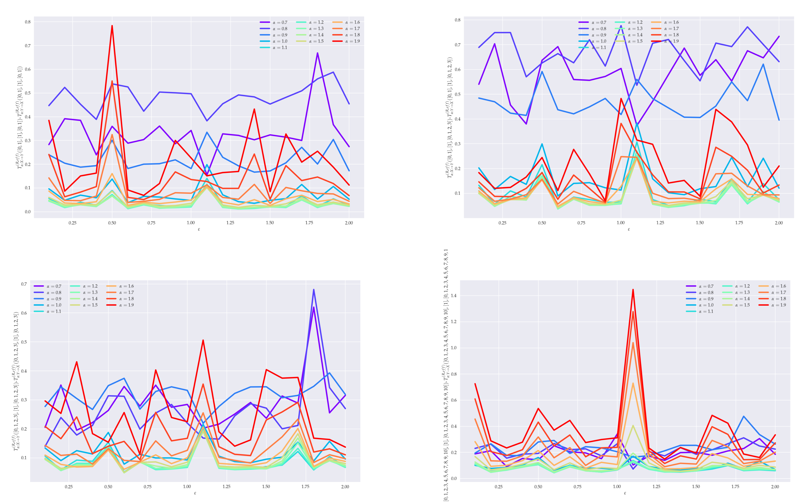
5. Analysis of Effective RTE for Coupled GARCH($1,1$) Processes

In this section, we use Estimator (11) for Rényi’s entropy to compute effective RTE (9) between coupled GARCH($1,1$) processes (13) and (14). The calculations are performed directly on log-returns (8) rather than on amplitudes. A typical dependence of RTE (7) on both $\alpha$ and the coupling strength $ϵ$ is depicted in Figure 1. Ensuing effective RTEs (9) with different Markov parameters are presented in Figure 2. In order to quantify the master–slave relationship in terms of information flow, the balance of flow (10) is calculated (see Figure 3). Respective standard deviations are depicted in Figure 4.

Based on experience with STE, one could anticipate that RTE $T_{\alpha ,X\to Y}^{R,\mathrm{eff}}$ (see also Figure 1) should increase with the growing value of the coupling parameter $ϵ$. This expectation is indeed confirmed for $\alpha \ge 1$. In fact, even though the trend is noisy, we can detect a clear upward drift. This can be interpreted as an increase in the information flow between central sectors of the underlying empirical distributions. On the other hand, for $\alpha <1$, the drift seems to be missing or even decreasing. This fact will be commented on shortly. The aforementioned type of behavior persists even when larger Markov parameters are considered, cf. Figure 2. The smallness of the $X\to Y$ information flow can be attributed to the indirect (nonlinear) coupling between X and Y.

From the results depicted in Figure 2, we can study how the increase in values of the Markov parameters in the respective time series influences the value of effective RTE. It can be observed that when historical values of the slave process Y are included, information flows improve (stabilizes) significantly. On the other hand, conditioning on the additional historical values of the master process X does not seem to change the information flows notably. However, for large histories, it stabilizes the results, as can be seen from the comparison of $(2,11)$ and $(11,11)$ in Figure 2.

The balance of effective transfer entropy presented in Figure 3 exhibits an increasing function of the coupling parameter $ϵ$ for $\alpha \ge 1$. Contrary to that, for $\alpha <1$, it is a stagnating or decreasing function with large fluctuations. The trend is most distinguishable for $(k,l)=(11,11)$. Thus, one can conclude that the deterministic behavior is bared by $\alpha >1$ and is stochasticity captured by $\alpha <1.$ Positive values of the balance of ERTE suggest higher information flows from the master process to the slave process than in the opposite direction. Therefore, $(11,11)$ confirms the omnipresent master–slave relationship.

Standard deviations of the balance of effective transfer entropy in Figure 4 reveal statistical stability of results for $\alpha >1$ in contrast to regime $\alpha <1$. The typical size of fluctuations in the latter case is about $5-10$ times larger than in the previous one. However, the results show instability in the results for various strengths of interaction among the time series $ϵ$. We admit that this is an effect of the insufficient size of datasets or missing statistics of datasets.

6. Conclusions

6.1. Summary

In this paper, we performed extensive computer calculations of the novel method to calculate Rényi’s transfer entropy that was applied to a coupled GARCH time series. We performed analogous analysis on the surrogate datasets. Based on that, we calculated the statistics of the balance of effective Rényi transfer entropy.

Analysis of the two-dimensional GARCH process where one dimension influences the latter using Rényi’s transfer entropy using the nearest order estimators provides insight into the flow of information within the system. Transfer entropy expectably increases with the increasing strength of the interaction, and the rate increases with the increasing indices of memory. Particularly, it increases with the memory of the time series where the interaction is heading. This observation follows for effective transfer entropy and the balance of effective transfer entropy.

6.2. Perspectives and Generalizations

Transfer entropy is a powerful tool to reveal the strength and direction of information flow in a time series. In combination with the effective use of computer power and modern advancements in the mathematical theory of entropy calculation, it is a better tool to investigate nonlinear causality than the Granger test that is limited to Gaussian time series with linear causality. The advantage of using Rényi’s entropy with parameter $\alpha$ is its ability to detect informational flow during extreme events, such as sudden jumps. This is because Rényi’s entropy gives an emphasis on the tails or the center of the probability distribution.

Using the complex algorithm on financial datasets can be a potent tool to reveal information flows among, e.g., different stocks or other valuable assets. It can be also used as a precursor of instability or critical behavior in international markets.

References

1. Pearl, J. Causality; Cambridge University Press: Cambridge, UK, 2009. [Google Scholar]
2. Schreiber, T. Measuring Information Transfer. Phys. Rev. Lett. 2000, 85, 461–464. [Google Scholar] [CrossRef] [PubMed] [Green Version]
3. Barnett, L.; Barrett, A.B.; Seth, A.K. Granger Causality and Transfer Entropy Are Equivalent for Gaussian Variables. Phys. Rev. Lett. 2009, 103, 238701. [Google Scholar] [CrossRef] [PubMed] [Green Version]
4. Lungerella, M.; Ishigoro, K.; Kuniyoshi, Y.; Otsu, N. Methods for quantifying the causal structure of bivariate time series. Prog. Neurobiol. 2007, 77, 1–37. [Google Scholar] [CrossRef] [Green Version]
5. Jizba, P.; Kleinert, H.; Shefaat, M. Rényi’s information transfer between financial time series. Physica A 2012, 391, 2971–2989. [Google Scholar] [CrossRef] [Green Version]
6. Leonenko, N.; Pronzato, L.; Savani, V. A class of Rényi information estimators for multidimensional densities. Ann. Stat. 2008, 36, 2153–2182. [Google Scholar] [CrossRef]
7. Rényi, A. On measures of entropy and information. Proc. Fourth Berkeley Symp. on Math. Statist. Prob. 1961, 1, 547–561. [Google Scholar]
8. Rényi, A. Selected Papers of Alfred Rényi; Akademia Kiado: Budapest, Hungary, 1976; Volume 2. [Google Scholar]
9. Jizba, P.; Arimitsu, T. World According to Rényi: Thermodynamics of Multifractal Systems. Ann. Phys. 2004, 312, 17–57. [Google Scholar] [CrossRef]
10. Beck, C.; Schlögl, F. Thermodynamics of Chaotic Systems; Cambridge Nonlinear Science Series (Book 4); Cambridge University Press: Cambridge, UK, 1995. [Google Scholar]
11. Paluš, M.; Hlaváčkovxax-Schindler, K.; Vejmelka, M.; Bhattacharya, J. Causality detection based on information-theoretic approaches in time series analysis. Phys. Rep. 2007, 441, 1–46. [Google Scholar]
12. Marschinski, R.; Kantz, H. Analysing the Information Flow Between Financial Time Series. Eur. Phys. J. B 2002, 30, 275–281. [Google Scholar] [CrossRef]
13. Samuelson, P.A. Rational Theory of Warrant Pricing. Ind. Manag. Rev. 1965, 6, 13–31. [Google Scholar]
14. Keylock, C.J. Constrained surrogate time series with preservation of the mean and variance structure. Phys. Rev. E 2006, 73, 036707. [Google Scholar] [CrossRef] [PubMed]
15. Dobrushin, R.L. A simplified method of experimentally evaluating the entropy of a stationary sequence. Teor. Veroyatnostei Primen. 1958, 3, 462–464. [Google Scholar] [CrossRef]
16. Vašíček, O. A test for normality based on sample entropy. J. Roy. Statist. Soc Ser. B Methodol. 1976, 38, 54–59. [Google Scholar]
17. Kantz, H.; Schreiber, T. Nonlinear Time Series Analysis; Cambridge University Press: Cambridge, UK, 2010. [Google Scholar]
18. Engle, R.F. Autoregressive Conditional Heteroscedasticity with Estimates of the Variance of United Kingdom Inflation. Econometrica 1982, 50, 987–1007. [Google Scholar] [CrossRef]
19. Bollerslev, T. Generalized Autoregressive Conditional Heteroskedasticity. J. Econom. 1986, 31, 7–327. [Google Scholar] [CrossRef] [Green Version]
Figure 1. Transfer entropy T α , X Y R ( 2 , 7 ) T ( R ) α , X Y ( [ 0 , 1 ] , [ 1 ] , [ 0 , 1 , 2 , 3 , 4 , 5 , 6 ] ) , where X and Y are GARCH processes described in Section 4. The coupling strength ϵ { 0.1 , 0.2 , , 2 } is on the horizontal axis, and the transfer entropy is on the vertical axis. Each graph represents a different value of α { 0.7 , 0.8 , , 1.9 } .
Engproc 05 00033 g001
Figure 2. Effective transfer entropy T α , X Y R , eff ( k , l ) T ( R ) α , X Y ( [ 0 , 1 , , k 1 ] , [ 1 ] , [ 0 , 1 , , l 1 ] ) , where ( k , l ) = ( 2 , 2 ) , ( 2 , 4 ) , ( 4 , 2 ) , ( 4 , 4 ) , ( 2 , 11 ) , ( 11 , 11 ) from left to right and from top to bottom. The coupling parameter ϵ is on the x-axis.
Engproc 05 00033 g002
Figure 3. Balance of effective transfer entropy T α , X Y R , bal eff ( k , l ) for ( k , l ) = ( 2 , 2 ) , ( 2 , 4 ) , ( 4 , 2 ) , ( 4 , 4 ) , ( 2 , 11 ) , ( 11 , 11 ) from left to right and from top to bottom. Coupling parameter ϵ is on the x-axis.
Engproc 05 00033 g003
Figure 4. Standard deviation of the balance of effective transfer entropy T α , X Y R , bal eff ( k , l ) for ( k , l ) = ( 2 , 2 ) , ( 2 , 4 ) , ( 4 , 4 ) , ( 11 , 11 ) from left to right and from top to bottom. With ϵ on the x-axis.
Engproc 05 00033 g004
Publisher’s Note: MDPI stays neutral with regard to jurisdictional claims in published maps and institutional affiliations.