Proceeding Paper

Improved Output Gap Estimates and Forecasts Using a Local Linear Regression †

Department of Economics, Paderborn University, Warburger Str. 100, 33098 Paderborn, Germany
Presented at the 7th International Conference on Time Series and Forecasting, Gran Canaria, Spain, 19–21 July 2021.
Eng. Proc. 2021, 5(1), 32; https://doi.org/10.3390/engproc2021005032
Published: 30 June 2021
(This article belongs to the Proceedings of The 7th International Conference on Time Series and Forecasting)

Abstract

:
The output gap, the difference between potential and actual output, has a direct impact on policy decisions, e.g., monetary policy. Estimating this gap and its further analysis remain the subject of controversial debates due to methodological problems. We propose a local polynomial regression combined with a Self-Exciting Threshold AutoRegressive (SETAR) model and its forecasting extension for a systematic output gap estimation. Furthermore, local polynomial regression is proposed for the (multivariate) OECD production function approach and its reliability is demonstrated in forecasting output growth. A comparison of the proposed gap to the Hodrick–Prescott filter as well as to estimations by experts from the FED and OECD shows a higher correlation of our output gap with those from those economic institutions. Furthermore, sometimes gaps with different magnitude and different positions above or below the trend are observed between different methods. This may cause competing policy implications which can be improved with our results.

1. Introduction

Since the influential work of [1], the output gap and its reliability have been widely discussed. Also, the importance of gap estimations for “conjunctural and monetary policy analysis” ([2], p. 2) is undisputed. The difficulties in the estimation of potential output are summarized by [3]. They distinguish three methods for its estimation: (i) statistical, (ii) production function and (iii) structural approaches. Ref [2] show that some statistical methods produce unreliable real-time estimates of the gap. These unreliable output gap estimates have induced unfavorable monetary policy activities, as [4] demonstrate for the UK. Thus, monetary policy recommendations need to be treated carefully as they depend heavily on the estimation method used for potential output.
The following four reasons for instable output gap estimations: (i) influence of first estimates on policy decisions, (ii) forecast errors, (iii) data revisions and (iv) varying decompositions of trend and cycle are identified by [5]. We focus on reducing the effects of (iv) by applying a new decomposition method and of (ii) by using more information, e.g., a regime-switching SETAR model. Furthermore, higher correlations of the recent proposal with output gaps from policy institutions and an improvement in the accuracy of output growth forecasts using the new output gap underline its reliability.
Since no true output gap exists one must rely in accordance with [6] on estimates without having an unambiguous definition from theory. Their paper summarizes numerous methods used to estimate the output gap, e.g., the Hodrick–Prescott (HP) filter, the [7] filter, and the [8] (BN) decomposition (see [9]). They distinguish between univariate time series methods and multivariate methods. Although multivariate methods process information from additional explanatory variables, ref [6] conclude that no multivariate model outperforms its univariate competitors. One of the most widely used methods for output gap estimations, employed e.g., by the European Commission (EC) and (indirectly) by the OECD, is the HP filter introduced by [10]. Using this penalized spline smoother results in very different gaps depending on the arbitrarily selected smoothing parameter λ ([1]), yielding somewhat arbitrary, either negatively or positively, output gaps [11]. Recently, the HP filter is criticized by [12] for causing problems at an unknown amount of boundary points. This becomes obvious once new data is available, which results in significant output gap revisions and reduces real-time reliability.
As mentioned by [13], many detrending methods perform poorly at time series endpoints, which results in output gaps that are sensitive to large revisions. This is also proposed by [1], who argue that the vast majority of output gap revisions are attributable to the boundary problems of detrending methods. This view contrasts with the expectation that data revisions are the primary source of uncertainty, whereas in line with [2] model and estimation uncertainty are much smaller. Further discussions on improvements of the FED output gap estimates and purely statistical methods over the last decades can be found in [13]. Nevertheless, they also confirm the poor reliability of solely statistical methods over the whole period and add that the accuracy of output gap estimates depends on the period under investigation, while the last decade eases gap estimation.
In order to estimate a reliable output gap accurately, an identification of trend and cycle is a prerequisite ([5]) and needs to be combined with the systematic analysis of the gap component. Therefore, any analyses need to provide additional information that can be used to estimate a more precise output gap. To use all available information in the sense of applying a two-sided filter, the local polynomial regression of [14] may be a better alternative for estimating the output gap. This method in its local linear (LLR) version also improves the estimation quality at boundary points, since an asymmetric boundary kernel is introduced to enhance the estimation quality at time series endpoints (real-time reliability). Moreover, the LLR allows for short-range dependence between trend and cyclical movements as required by [9] who analyze the revision properties of the BN decomposed output gap. The use of a (semi-)SETAR model provides additional information for the output gap. We then extend the method to forecast output gaps. Moreover, the univariate LLR of [14] is extended to multivariate analysis to examine the contribution of multivariate methods. Besides introducing this methodology, we also compare the gaps produced using the LLR with those using the HP filter for (i) statistically based estimations and (ii) the production function approach used by the OECD. Finally, the output gap estimated by experts from the FED and OECD is used as a benchmark. However, since no original gap exists, the comparison with external criteria on the appropriateness of the gap is difficult.
Section 2 presents the nonparametric LLR. Section 3 shows its application and compares it to the HP gap. Section 4 combines output gaps and semi-SETAR models by comparing different methodologies to those of the FED and the OECD by extending the univariate LLR approach to a multivariate method. Section 5 shows the predictive power of the new gap for output growth. Section 6 concludes.

2. Local Linear Regression

In the introduction, the HP filter is criticized for its suboptimality at boundary points. The LLR has automatic boundary correction [15], ensuring that asymptotic properties of the estimators in the interior still hold at boundary points. We focus on the estimation quality at these points and use an asymmetric boundary kernel to obtain stable boundary estimates, which are the key to obtaining reliable real-time output gap estimates. Ref [14] use an additive component model:
Y t = m ( x t ) + ξ t ,
where Y t is a sequence of macroeconomic time series with time t = 1 , , T ,   x t = t / T denotes the rescaled time, m ( x ) is some smooth function and ξ t denotes a zero mean stationary process.
Thus, a data-driven local polynomial estimator for the smooth trend function is used in line with [14] without any parametric assumptions on ξ t . Under the assumption of short-range dependence the authors use the following Equation (2) for estimating the trend m ( x t ) by minimizing the locally weighted least squares:
Q = t = 1 T { y t j = 0 p β j ( x t x ) j } 2 W ( x t x h ) ,
where W ( u ) = C µ ( 1 u 2 ) µ 𝟙 [ 1 , 1 ] ( u ) ,   µ = 0 ,   1 ,   is the weight function (a second order kernel on [ 1 ,   1 ] ) and h is the (relative) bandwidth. In Equation (2) the bandwidth determines the smoothness of the trend and is the counterpart to HP’s λ . Minimizing Equation (2) yields any v -th derivative of m ( x ) , defined as m ( v ) ( x )   ( v p ) . If p ν is odd, the linear smoother m ^ ( v ) ( x ) has automatic boundary correction and the bias is of order k ν . We use the Epanechnikov kernel as the weight function, which is optimal in the MSE sense. The resulting trend estimates are m ^ ( v ) ( x ) = v ! β ^ v , where v = 0 ,   1 ,   ,   p . Since the local linear estimator, where p = 1 , results in the most stable boundary estimates (for two-sided filters), it seems a logical choice for estimating the output gap. In order to estimate the bandwidth in a data-driven manner, we follow [14], where the bandwidth is estimated by minimizing the asymptotic mean integrated squared error (AMISE):
A M I S E ( h ) = h 2 ( k v ) I [ m ( k ) ] β 2 [ k ! ] 2 + 2 π c f ( d b c b ) R ( K ) T h 2 v + 1 .
The corresponding optimal bandwidth h for estimating m ( x ) on [ 0 ,   1 ] is chosen using:
h A = ( 2 v + 1 2 ( k v ) 2 π c f [ k ! ] 2 ( d b c b ) R ( K ) I [ m ( k ) ] β 2 ( v , k ) ) 1 ( 2 k + 1 ) T 1 / ( 2 k + 1 ) ,
where I [ m k ] = c b d b [ m ( k ) ( x ) ] 2 d x ,   β ( v , k ) = 1 1 u k K ( u ) d u , and R ( K ) = 1 1 K 2 ( u ) d u , and K is the asymptotically equivalent kernel in the interior. Furthermore, v is the order of the derivative and k = p + 1 , so that m is k -times continuously differentiable. c f = f ( 0 ) is the value of the spectral density of ξ t at the origin, with f ( λ ) = 1 / 2 π l = γ ξ ( l ) e i l λ , π λ π . The dependence structure is fully captured by the bandwidth. The values c b and d b can be chosen to select the bandwidth using only observations between these bounds. Details of the data-driven IPI are described in [15]. To address the criticism of [12,16], an asymmetric boundary kernel is used to weight the boundary points and the bandwidth at the boundary is kept constant such that the asymptotic properties at the boundary are the same as in the interior [17].

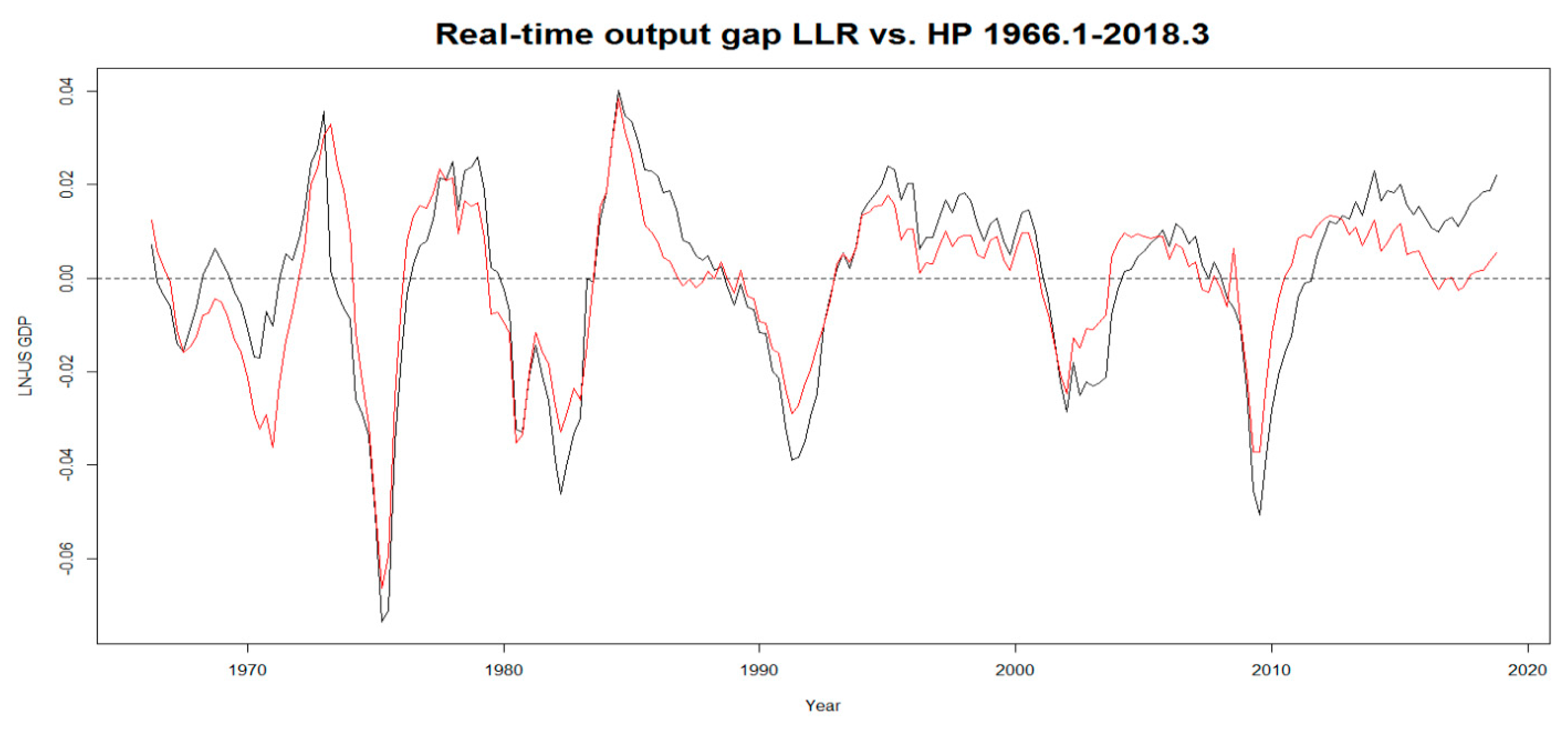
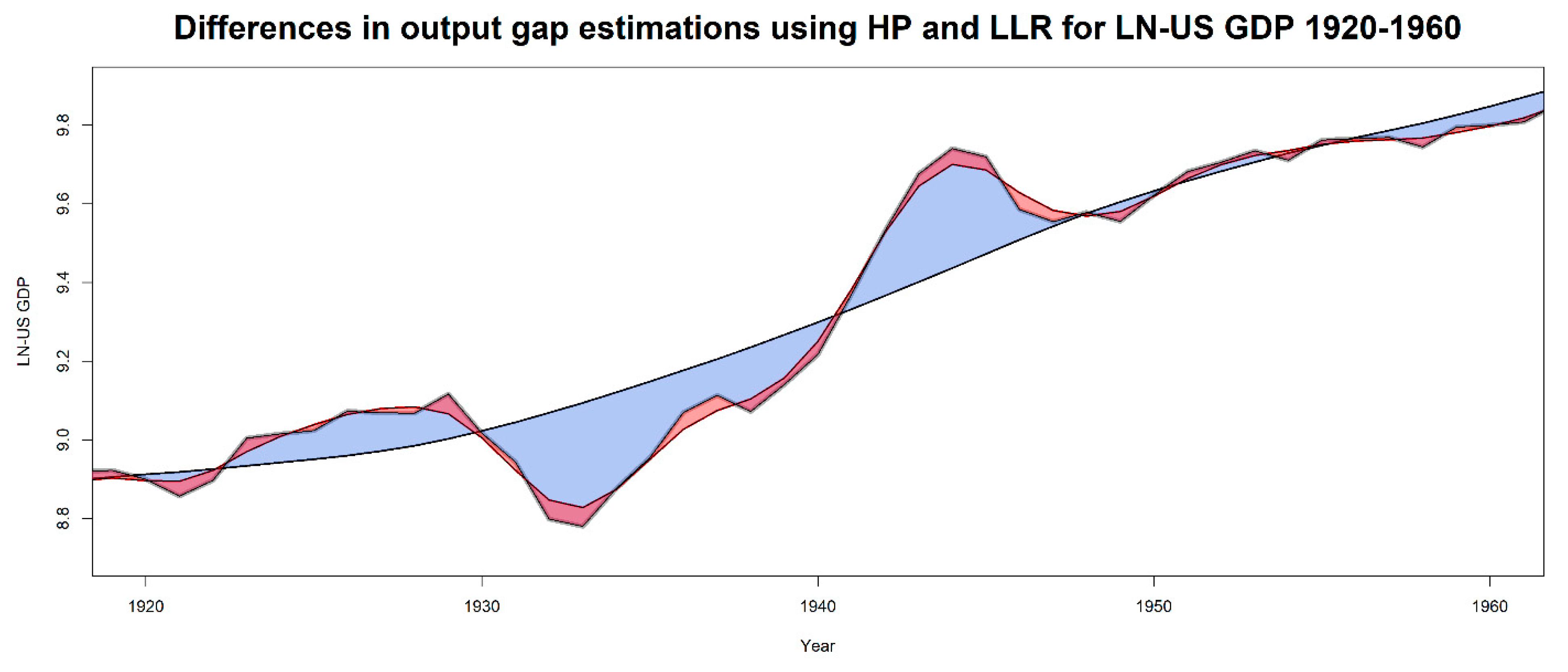
3. Output Gap Estimation Using the LLR

In this section, the LLR is used to estimate the output gap for the US economy without any parametric model assumptions of the output gap component. Therefore, quarterly US GDP vintages from 1947.1 to 2018.3 and annual US GDP from 1790 to 2018 by [18] are used. To contrast our results with those of [1,19], we follow their definitions. Thus, the final estimate of the output gap is defined as the detrended last available vintage (2018.3). Using the LLR for every vintage and collecting each endpoint estimation delivers a new time series that is defined as “the real-time estimate of the output gap” ([1], p. 571). As in [19], the last 2 years are not used to ensure that the comparison is not biased by the last vintages.
Figure 1 shows the real-time output gap estimates of the LLR compared to those of the HP filter ( λ = 1600 ) for quarterly US GDP data. The HP filter and the LLR could be quite similar if λ is chosen correctly, which can also be detected in the resulting output gaps. Nevertheless, these approaches sometimes yield very different output gaps. In some cases, only the magnitude of the gaps differs, whereas in others the sign is contradicting. The HP gap is slightly smaller for the period from 1966.1 to 2018.3. This is obvious especially since the 2000s. These observations confirm the analysis of [1], where different detrending procedures yield various output gaps.
An even more stable real-time estimation of the gap is possible by using the LLR, since the trend is estimated appropriately with regard to the data-driven degree of smoothing and the introduced boundary correction increases the reliability of the output gap. The poor performance of the HP filter during periods of increased cyclical variation is examined by [20,21]. They conclude that using an unreliable detrending method such as the HP filter results in crises that are shown to be less intense than they actually are because most changes are attributed to trend movements. This presumable underestimation of the output gap using the HP filter is evident in Figure 2, where the gaps are shown for the Great Depression using data from 1790 to 2018. In this figure, the LLR (black) and the HP trend with λ = 6.25 (red) are shown for annual observations (grey line) from 1920 to 1960. The HP filter gap (red area) is significantly smaller than that estimated with the LLR (blue area). This may be a hint for the underestimation properties of the gap proposed by [20,21]. It is important to note that the amplitude of the HP filter can be adjusted using different values of λ . Nevertheless, for the LLR the bandwidth estimation is data-driven, so the arbitrary choice of λ is not necessary. To summarize, the data-driven selection and the stable and automatic boundary correction demonstrate the advantages of the LLR. The effects due to parameter, model and data uncertainty in the sense of [2] are per definition lower using the HP filter, but these smaller effects may not reflect the true output gap.
Since crises are unusually volatile transitory events, it is expected that the HP filter, which assumes a constant signal-to-noise ratio, performs less reliable in those periods. Although the IPI captures heteroscedastic events due to minimization of the AMISE, we improve the LLR by implementing a version that is able to leave those periods out for bandwidth selection.
The possible underestimation heavily influences monetary policy by, e.g., central banks, that in turn under- or overshoot with their interventions. Moreover, the different gap estimations influence the timing of policy actions. The HP filter has a similar disadvantage as one-sided filters. [16] argues in the setting of bandpass filtering that the underestimation of the output gap using these methods is a substantial error. A similar analysis for the period of the financial crisis around 2007/2008 shows that the estimated output gaps get smaller after the 2000s. As expected, the gap is significantly smaller than that estimated during the Great Depression, independent of the detrending approach, with neither method showing a significant gap for the recent period.
Various sources of uncertainty for gap estimation are identified by [2]. To analyze parameter uncertainty and parameter instability, we compare the final estimates and the real-time estimates of the output gap in Figure 3, which compares the real-time LLR gap (black) to the final LLR gap (green). Further, the real-time gap estimated with the HP filter (red) is compared to the final HP gap (blue). The differences between the real-time LLR gap (black) and the final LLR gap (green) partly reflect these different uncertainties. It is argued that a higher correlation between final and real-time estimation shows a lower level of revisions [2]. The calculated correlation for the LLR is 0.2949 and that for the HP filter is 0.5083 . This discrepancy can be explained by the data-driven nature of the LLR, where the bandwidth changes slightly with every new observation point because the bandwidth depends on the sample size T (Equation (3)). By contrast, the smoothing parameter for the HP filter is fixed at λ = 1600 , which causes no additional revisions to the gap estimates. Consequently, the correlation for the HP filter gap is higher per definition. However, the revision properties show that the LLR is appropriate for the ex post analysis of the output gap.

4. Models for the Output Gap Component

The proposed AMISE-optimal decomposition may identify a more systematic cyclical component that needs to be analyzed during the further estimation of the output gap. Therefore, SETAR is used to further analyze the characteristics of the two different (LLR vs. HP) output gap series.

4.1. Semi-SETAR Model

To verify that the deterministic LLR combined with a further model for the gap component produces a more stable output gap, we fit different SETAR(k,p,d) models, as introduced by [22,23], to the residuals and their growth rates (LLR and HP gaps):
ξ ^ t = ϕ 0 ( j ) + ϕ 1 ( j ) ξ t 1 ϕ p ( j ) ξ t p + a t ( j ) ,   if   γ j 1 ξ t d < γ j
Residuals ξ ^ t are estimated by past realizations ξ t p and autoregressive coefficients ϕ p ( j ) such that the threshold variable ξ t d with d depicting the delay parameter lies in the range of γ j 1 up to γ j dividing the domain of ξ t d into j regimes. a t ( j ) are white noise errors. Trend and cycle are estimated using the LLR and HP filter and gaps are further analyzed with a SETAR model (We focus on the results for annual data as they are mostly used for cyclical analysis, see [2]). This modified and more systematic output gap identification has its merits for accurately timed policy actions, as additional information reduces problems affiliated with unsuitable policy activities [4].
In line with [14], we allow for two different regimes ( j = 2 ) which are separated by the threshold zero in a high regime (HR) for expansions and a low regime (LR) for recessions. Moreover, different orders p = 1 ,   2 ,   3 of the AR part are tested and the delay parameter is set to d = 0 . The results are displayed in Table S1 in the supplement material. It is evident that the coefficients are larger for the SETAR models fitted to the LLR output gap. Both coefficients are significantly different from zero. Whereas ϕ 1 , L L R L R = 0.9235 implies that the next observation will be roughly the same within the same regime, ϕ 1 , H P L R = 0.3345, which is much lower in magnitude, implies a much lower probability of similarity to the last observation Y t 1 . Thus, the LLR shows more systematic and larger gaps. By contrast, the HP filter gap implies more short-lived differences between actual and potential output. Using the 0.04 gap observed in 2010 leads to a gap of LLR that is three times the magnitude of that calculated using the HP based SETAR model (in absolute terms) and it lasts for a longer period when calculated with the LLR. The growth rates are analyzed in Table S2 in the supplements. The additional information provided by the LLR shows a long-lasting and significant expansion regime resulting in more accurately timed intervention of monetary policy makers (central banks). This drawback of the HP filter is ascribed to the arbitrarily selected smoothing parameter.

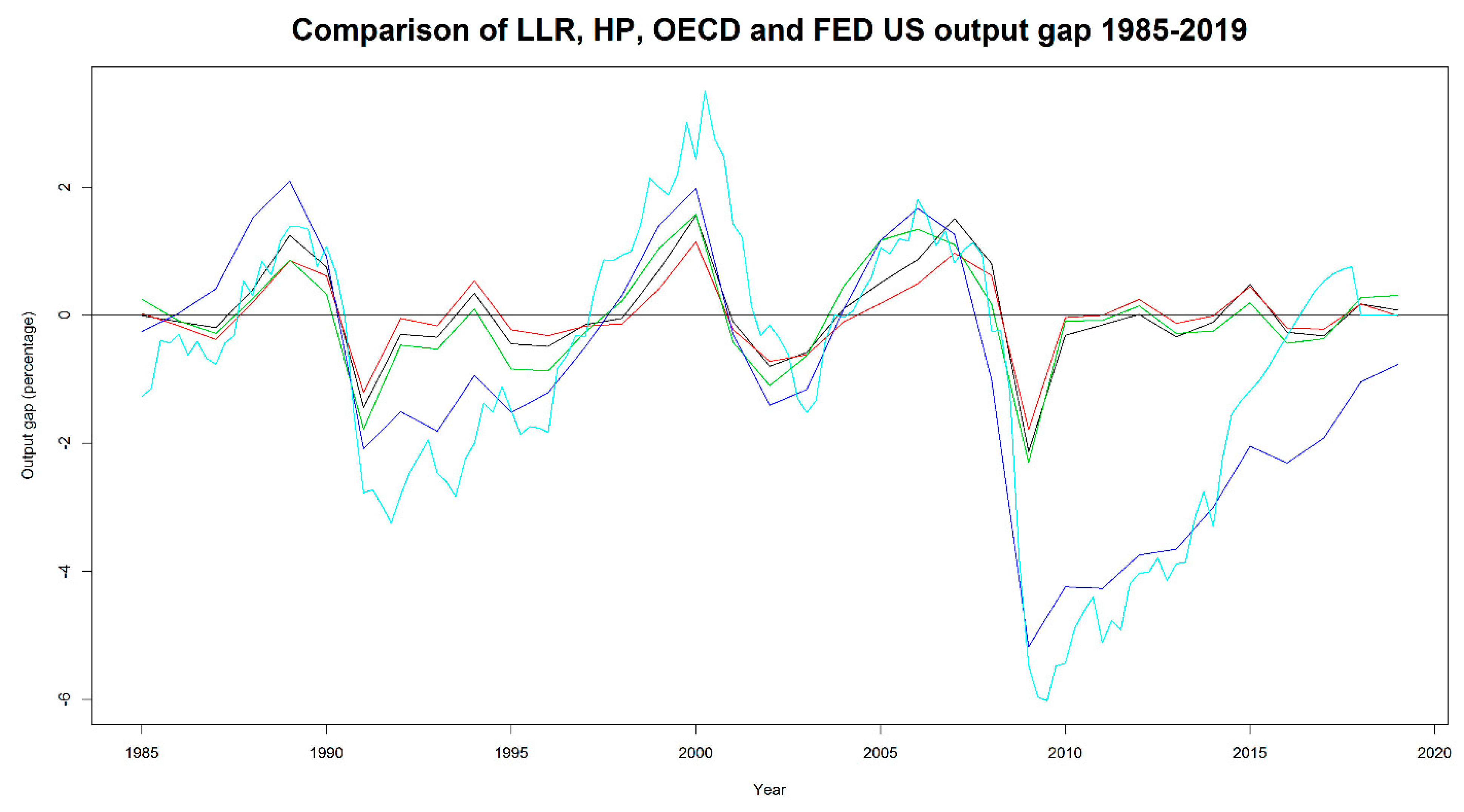
4.2. The OECD Approach and the Multivariate LLR

Since the true output gap is not observable, a valuation is difficult but a comparison with a methodological framework used by experts is straightforward. To demonstrate the performance of the LLR output gap estimations, we compare it to the output gap calculated by the OECD Economics Department. Using a Cobb–Douglas production function approach, [24] calculate potential output by using the trend components of labor efficiency (LE), a population between 15 and 74 (POP), and labor force participation rate between 15 and 74 (LFPR) obtained with a cyclical adjustment and the HP filter, with λ = 100 . The unemployment rate is considered and filtered through the Kalman filter, where the productive capital stock (PK) enters the estimation without detrending. Following Equation (4) of [24], potential GDP (PGDP) is estimated by:
P G D P = [ L E · P O P · L F P R 100 · ( 1 U N R 100 ) ] α · ( P K ) ( 1 α ) .
To compare the OECD gap to the LLR gap, we adjust the estimation method of [24] by replacing the HP components in their Cobb–Douglas production function in our Equation (6) by the trend obtained using the LLR. Therefore, we extend the LLR to a multivariate approach. Afterwards, we determine potential output and finally the output gap. Figure 4 displays the OECD output gap approach using the LLR for detrending (green) together with the OECD gap using the HP filter (blue). Again, both estimated output gaps are quite similar and the magnitude is not significantly different, except during the Great Recession, where the OECD gap shows a much larger cycle. From 2008 onwards, the amplitude of the HP-filtered output gap is much larger than that of the LLR-based gap. Surprisingly, these results show that the LLR seems to have a higher variability than the HP trend since the Great Recession, which may be explained by additional cyclical adjustment used in [24]. However, the LLR needs no cyclical adjustment before detrending, is fully data-driven and more stable at boundary points in real-time applications.

4.3. Comparison of Univariate EC and Multivariate OECD Approach

Multivariate methods, like the OECD production function approach, do not significantly enhance the quality of output gap estimation but impose additional structural assumptions [6]. Univariate time series methods, as used by the EC and the LLR, perform quite reasonably. To compare univariate and multivariate methods and to show the performance of the LLR in both types of applications, Figure 4 displays the gaps using the LLR (black) and the HP filter (red) for the final time series and the output gaps using the production function approach with the LLR (green) and the HP filter (blue). The output gap estimates from the FED (turquoise) are displayed as a benchmark in accordance with [13]. Obviously, both final univariate output gaps yield quite similar results (as for quarterly data). The gaps produced using the OECD approach are larger, although both multivariate gaps show similar dynamics. Those dynamics are also in line with the FED output gap. Surprisingly, the differences between the FED output gap and the OECD HP gap increase after 2014. It is important to mention that the frequency of the FED data is quarterly, thus the variability is larger than in the other series. However, using the HP filter and the additional cyclical adjustments of [24] produces a significantly larger gap than using the LLR. The LLR delivers output gap results in univariate and multivariate approaches that are in between those using the HP filter. Thus, the HP time series method may underestimate the gap while the HP OECD approach may overestimate it. This could be an argument in favor of the data-driven LLR, which is less arbitrary than the HP filter with regard to the degree of smoothness and produces more stable boundary estimates. As mentioned by [19], output gaps estimated by policy institutions provide a good benchmark to compare gaps. Thus, gaps from economic experts may be more reliable compared to purely statistical approaches [13]. They demonstrate that the FED use an evaluated and weighted average of statistical and structural methods. Table 1 shows the correlation coefficients for the LLR and HP based output gaps with those of the FED and the OECD. The correlation coefficients between the proposed LLR approach and the expert gaps are significantly higher than using the real-time HP filter gap. Using the LLR depicts the gaps estimated with economic expertise more reliably than using the HP filter. In other words, the LLR reflects the output gap benchmark provided by policy institutions more precisely than the HP filter.

5. Forecasting and Evaluating Output Gaps

Among others, ref [25] use forecasting methods to estimate revisions in potential growth. Since the semi-SETAR model is able to reproduce cyclical features in recessions and expansions, extending it to forecast gaps is straightforward.

5.1. Output Gap Forecasting Using the Semi-SETAR Model

We use the LLR and the SETAR model to forecast the output gap. Firstly, the trend is estimated and removed from the original observations (Equation (1)). Secondly, a SETAR model is fitted to the residuals (Equation (5)). Finally, the SETAR model is used for forecasting using the SETAR(2,3,0) model and quarterly US GDP data. The forecast horizon is set to five quarters ( k = 5 ), so the training set ranges from 1947.1 to 1966.1. The series are forecasted (in sample) by recursively updating the sample by one observation starting in 1966.1. To capture different uncertainties, we use a bootstrap method with n = 10,000 to forecast the future paths of US output [23]. The forecast results are depicted exemplarily for the sample ending 2017.3 (last in sample forecast) in Figure S1 in the supplements. Compared to the original observations, the semi-SETAR model is able to forecast the output gap quite well for the first year. Original observations and forecasts are nearly identical from 2017.3 to 2018.2 (The detailed results for every forecast value between 1966.1–2018.3 are available upon request). To validate the forecast performance, we calculate the mean absolute scaled error (MASE), which is M A S E = 0.5952 in this case. Thus, the semi-SETAR model improves forecast performance and delivers a reliable output gap forecast by including information from two regimes.

5.2. Predictive Power of the LLR Output Gap for Output Growth

Problems in evaluating the output gap due to a missing true gap can be overcome by the evaluation of the forecasting performance of the output gap for output growth [26]. use This idea is used by [19] by arguing for a negative correlation between gaps and future growth. They use the following equation to predict output growth using the estimated real-time gap:
y t + k y t = α + β c ^ t + ϵ t + k   | t ,
where y t + k y t is output growth, c ^ t is the estimated real-time output gap using either the LLR or HP filter and ϵ t + k   | t displays the forecast error. The forecast horizon is k = 1 , , 8 . Due to the trend-reverting properties, β < 0 is expected [19,26]. The OLS estimates show the expected signs for LLR- and HP-filtered gaps and are significantly negative for k = 1 , , 8 .
By comparing the relative RMSEs in Table 2, a small improvement in forecast accuracy is found using the LLR real-time gap. Surprisingly, the gains are higher the larger the forecast horizon is. Compared to the forecasting performance when using the HP gap, the LLR gap improves the forecast accuracy of output growth. A similar exercise can be carried out for inflation. However, in accordance with [13] output gaps usually do not improve inflation forecasts and are hence omitted.

6. Policy Implications and Conclusions

We argue for a more detailed and systematic output gap analysis by combining output gap estimation and SETAR models. Using this additional information, the improved estimation quality at boundary points and the LLR result in an improved estimation of the output gap compared to the standard HP-filtered gap. This is demonstrated by a comparison of both statistically based methods with those estimated with economic expertise by the OECD and the FED. The LLR output gap shows a higher correlation with the OECD and FED gap than the HP filter does. This is partly attributable to the data-driven selection of the bandwidth, which improves the disadvantage of the arbitrary selection in the HP filter. In addition, the HP time series filter attributes more originally cyclical fluctuations to the trend and leaves a too-small gap component, a misspecification that may impede an appropriate real-time gap estimation. Within the OECD approach, we observe the other extreme of a large output gap using the HP filter in combination with the production function approach. While the LLR is successfully extended to the multivariate production function approach, it performs similarly to the OECD method. Extending the semi-SETAR model improves output gap forecasts using additional information from different growth regimes. Using the proposed output gap for forecasting output growth, the LLR real-time gap performs better compared to the HP gap, in the sense that it has a larger predictive power for output growth. These results modify the timing and magnitude of monetary policy decisions as the new model allows a more reliable output gap estimation than the HP filter.

Supplementary Materials

The following are available online at https://www.mdpi.com/article/10.3390/engproc2021005032/s1. Table S1: Estimated model parameters for SETAR(k,p,d) model US GDP 1790-2018 using LLR and HP filter for the residuals. Table S2: Estimated model parameters for SETAR(k,p,d) model US GDP 1790-2018 using LLR and HP filter for the residual growth rates. Figure S1: SETAR(2,3,0) point forecast of the output gap (red dashed) together with the original data (black dotted) for 2017.3-2018.4 using the LLR for quarterly US GDP (black solid) 1947.1-2018.3.

Funding

This research did not receive any specific grant from funding agencies in the public, commercial or not-for-profit sectors.

Institutional Review Board Statement

Not applicable.

Informed Consent Statement

Not applicable.

Data Availability Statement

The data used in this study can be accessed through the following links:

Acknowledgments

I thank Thomas Chalaux for providing the data for the comparison and Lukas Wiechers for providing excellent research assistance. I also thank Frédérique Bec, Francisco Serranito, Camelia Turcu and the participants of the 7th Applied Macro-Econometrics Workshop in Paris and the 22nd INFER annual conference for their helpful comments and suggestions.

Conflicts of Interest

The author declares no conflict of interest.

References

  1. Orphanides, A.; van Norden, S. The Unreliability of Output-Gap Estimates in Real Time. Rev. Econ. Stat. 2002, 84, 569–583. [Google Scholar] [CrossRef] [Green Version]
  2. Marcellino, M.; Musso, A. The Reliability of Real Time Estimates of the Euro Area Output Gap. Econ. Model. 2010, 28, 1842–1856. [Google Scholar] [CrossRef] [Green Version]
  3. Coibion, O.; Gorodnichenko, Y.; Ulate, M. The Cyclical Sensitivity in Estimates of Potential Output; National Bureau of Economic Research Working Paper No. w23580; National Bureau of Economic: Cambridge, MA, USA, 2017. [Google Scholar]
  4. Nelson, E.; Nikolov, K. UK Inflation in the 1970s and 1980s: The Role of Output Gap Mismeasurement. J. Econ. Bus. 2003, 55, 353–370. [Google Scholar] [CrossRef]
  5. Grigoli, F.; Herman, A.; Swiston, A.; Di Bella, G. Output Gap Uncertainty and Real-Time Monetary Policy. Russ. J. Econ. 2015, 1, 329–358. [Google Scholar] [CrossRef] [Green Version]
  6. Álvarez, L.J.; Gómez-Loscos, A. A Menu on Output Gap Estimation Methods. J. Policy Model. 2018, 40, 827–850. [Google Scholar] [CrossRef] [Green Version]
  7. Baxter, M.; King, R.G. Measuring Business Cycles: Approximate Band-Pass Filters for Economic Time Series. Rev. Econ. Stat. 1999, 81, 573–593. [Google Scholar] [CrossRef]
  8. Beveridge, S.; Nelson, C.R. A New Approach to Decomposition of Economic Time Series into Permanent and Transitory Components with Particular Attention to Measurement of the Business Cycle. J. Monet. Econ. 1981, 7, 151–174. [Google Scholar] [CrossRef]
  9. Kamber, G.; Morley, M.; Wong, B. Intuitive and Reliable Estimates of the Output Gap from a Beveridge-Nelson Filter. Rev. Econ. Stat. 2018, 100, 550–566. [Google Scholar] [CrossRef] [Green Version]
  10. Hodrick, R.J.; Prescott, E.C. Postwar U.S. Business Cycles: An Empirical Investigation. J. Money Credit Bank. 1997, 29, 1–16. [Google Scholar] [CrossRef]
  11. De Brouwer, G. Estimating Output Gaps; Research Discussion Paper 9809; Reserve Bank of Australia: Sydney, Australia, 1998. [Google Scholar]
  12. Hamilton, J.D. Why You Should Never Use the Hodrick-Prescott Filter. Rev. Econ. Stat. 2018, 100, 831–843. [Google Scholar] [CrossRef]
  13. Edge, R.M.; Rudd, J.B. Real-Time Properties of the Federal Reserve’s Output Gap. Rev. Econ. Stat. 2016, 98, 785–791. [Google Scholar] [CrossRef]
  14. Fritz, M.; Gries, T.; Feng, Y. Growth Trends and Systematic Patterns of Booms and Busts—Testing 200 Years of Business Cycle Dynamics. Oxf. Bull. Econ. Stat. 2019, 81, 62–78. [Google Scholar] [CrossRef]
  15. Feng, Y.; Gries, T.; Fritz, M. Data-driven local polynomial for the trend and its derivatives in economic time series. J. Nonparametric Stat. 2020, 32, 1–24. [Google Scholar] [CrossRef]
  16. Watson, M.W. How Accurate Are Real-Time Estimates of Output Trends and Gaps? Econ. Q. 2007, 93, 143–161. [Google Scholar]
  17. Fritz, M.; Gries, T.; Feng, Y. Secular Stagnation? Is there Statistical Evidence of an Unprecedented, Systematic Decline in Growth? Econ. Lett. 2019, 181, 47–50. [Google Scholar] [CrossRef]
  18. Johnston, L.; Williamson, S.H. “What Was the U.S. GDP Then?”. Measuring Worth. 2019. Available online: http://www.measuringworth.org/usgdp/ (accessed on 15 June 2019).
  19. Quast, J.; Wolters, M.H. Reliable Real-Time Output Gap Estimates Based on a Modified Hamilton Filter. J. Bus. Econ. Stat. 2020, 1–17. [Google Scholar] [CrossRef]
  20. McCallum, B.T. Alternative Monetary Policy Rules: A Comparison with Historical Settings for the United States, the United Kingdom, and Japan; National Bureau of Economic Research Working Paper No. w7725; National Bureau of Economic: Cambridge, MA, USA, 2000. [Google Scholar]
  21. Pollock, D.S.G. Trend Estimation and De-Trending via Rational Square-Wave Filters. J. Econom. 2000, 99, 317–334. [Google Scholar] [CrossRef]
  22. Tong, H. Threshold Models in Nonlinear Time Series Analysisl; Time Series Analysis; Springer: Berlin, Germany, 1983. [Google Scholar]
  23. Grabowski, D.; Staszewska-Bystrova, A.; Winker, P. Generating Prediction Bands for Path Forecasts from SETAR Models. Stud. Nonlinear Dyn. Econom. 2017, 21, 1–18. [Google Scholar] [CrossRef]
  24. Chalaux, T.; Guillemette, Y. The OECD Potential Output Estimation Methodology; OECD Economics Department Working Papers No. 1563; OECD Publishing: Paris, France, 2019. [Google Scholar] [CrossRef]
  25. Blanchard, O.; Lorenzoni, G.; L’Huillier, J.P. Short-Run Effects of Lower Productivity Growth. A Twist on the Secular Stagnation Hypothesis. J. Policy Model. 2017, 39, 639–649. [Google Scholar] [CrossRef] [Green Version]
  26. Nelson, C.R. The Beveridge-Nelson Decomposition in Retrospect and Prospect. J. Econom. 2008, 146, 202–206. [Google Scholar] [CrossRef]
Figure 1. Real-time output gap estimation for quarterly US GDP data from 1966.1 to 2018.3 using the local linear regression (black) and the HP filter (red).
Engproc 05 00032 g001
Figure 2. Estimation of the LLR (black) and the HP trend (red) with its corresponding gap estimations (blue area for LLR gap and red area for HP gap) and the original observations (grey) for US GDP from 1920 to 1960.
Engproc 05 00032 g002
Figure 3. Real-time LLR (black) and final LLR (green) output gaps compared to real-time HP (red) and final HP (blue) output gaps estimation for quarterly US GDP data from 1966.1 to 2018.3.
Engproc 05 00032 g003
Figure 4. Comparison of univariate LLR (black) and HP filter (red) output gap with the OECD output gap using the LLR (green) and the HP filter (blue) together with the FED output gap (turquoise).
Engproc 05 00032 g004
Table 1. Correlation between real-time LLR and HP gaps with ex post gaps from policy institutions.
Output GapFEDOECD
LLR0.64880.7071
HP0.50710.5678
Table 2. Relative RMSEs for output growth forecasts evaluation using LLR and HP real-time gaps.
Horizon12345678
LLR/HP0.99991.00311.00741.00580.99580.98420.97170.9612
Publisher’s Note: MDPI stays neutral with regard to jurisdictional claims in published maps and institutional affiliations.

