Time-Series of Distributions Forecasting in Agricultural Applications: An Intervals’ Numbers Approach ^†

Abstract

This work represents any distribution of data by an Intervals’ Number (IN), hence it represents all-order data statistics, using a “small” number of L intervals. The INs considered are induced from images of grapes that ripen. The objective is the accurate prediction of grape maturity. Based on an established algebra of INs, an optimizable IN-regressor is proposed, implementable on a neural architecture, toward predicting future INs from past INs. A recursive scheme tests the capacity of the IN-regressor to learn the physical “law” that generates the non-stationary time-series of INs. Computational experiments demonstrate comparatively the effectiveness of the proposed techniques.

1. Introduction

There is a long-term interest in extending the fourth industrial revolution (Industry 4.0) to agricultural production [1]. Regarding viticulture, in particular, the interest is in minimizing the human presence in the vineyard during production. In the aforementioned context, the accurate prediction of the grape maturity is critical in order to timely engage both human labor and equipment for harvest. Newly introduced technologies from associated areas such as the Internet of Things (IoT), Big Data, and Artificial Intelligence (AI) can be combined with autonomous robotic systems in order to collect and interpret data, monitor and evaluate crop status, and automatically plan effective and timely interventions. An early in-field assessment of fruit maturity level and therefore an estimation on harvest time has the potential to enable sustainable farming by balancing between economy, ecology, and optimal crop quality [2]. However, the development of autonomous robots for agricultural applications faces the daunting scale of the data involved [3]. Our special interest here is in the prediction of grapes maturity level, intended to be integrated into an autonomous grape-harvester robot [4].

Fruit maturity can be studied as a time-series, where the sequence of maturity data, m₁, m₂, …, m_D is indexed in time. The objective is to predict future fruit’s maturity level. A number of different models have been used including linear ones such as classic autoregressive (AR), moving average (MA), autoregressive moving average (ARMA), and autoregressive integrated moving average (ARIMA) models; however, those models typically assume stationary time-series [5,6], and they may fail with non-stationary time-series regarding maturity, unless a very high order linear model is used to gain an insight into the system and its underlying laws. The latter needs extensive learning which calls for long processing time as well as computational resources. Therefore, nonlinear models, such as Neural Networks (NN), have been proposed to counter forecasting problems [7,8,9]. The most straightforward approach for an NN model to learn a time-series is to provide the samples in time to the input of the NN. However, if the time-series are complex, then more past samples are needed; the latter usually results in a complex system of multiple inputs and weights.

This paper uses Intervals’ Numbers (INs) for predicting the maturity of grapes based on real-world measurements by a parametric IN-regressor model implementable by a neural network architecture. Note that INs have originally been introduced, under the name Fuzzy Intervals’ Numbers (FINs), in the context of fuzzy set theory [10]. The interpretation of INs was later extended, in the context of the Lattice Computing (LC) information processing paradigm [11]. In particular, an IN has been defined as a mathematical object that can be interpreted either as a fuzzy interval or as a distribution of samples; the latter interpretation implies that an IN can potentially represent all-order statistics [11]. The mathematical properties of the set of INs have been studied for a long time. An algebra of INs has been established [10,12,13]. INs have been employed in logic and reasoning applications [14,15]. Furthermore, they have been employed in interpolation/extrapolation applications [16].

INs have already been applied to time-series classification applications regarding electroencephalography (EEG) signals [17]. Recently, INs have been employed toward predicting the maturity of grapes [18]. This work is a follow-up of [18] with the following novelties: first, additional computational experiments are carried out using (1) the previous three and four INs to predict a future IN, (2) fewer data for training; second, a recursive scheme here demonstrates an IN-regressor’s capacity to learn the physical “law” that generates the non-stationary time-series of INs regarding grape maturity; third, the problem of time-series forecasting in agriculture is described, in mathematical terms, as a non-stationary time-series forecasting problem thus bringing INs to the foreground as an object for time-series processing in other domains with the advantage that an IN represents a distribution of data including all-order data statistics.

The layout of the paper is as follows: Section 2 presents two IN-regressor models for prediction. Section 3 details experimental application results. Finally, Section 4 summarizes our contribution, and it discusses potential future work extensions.

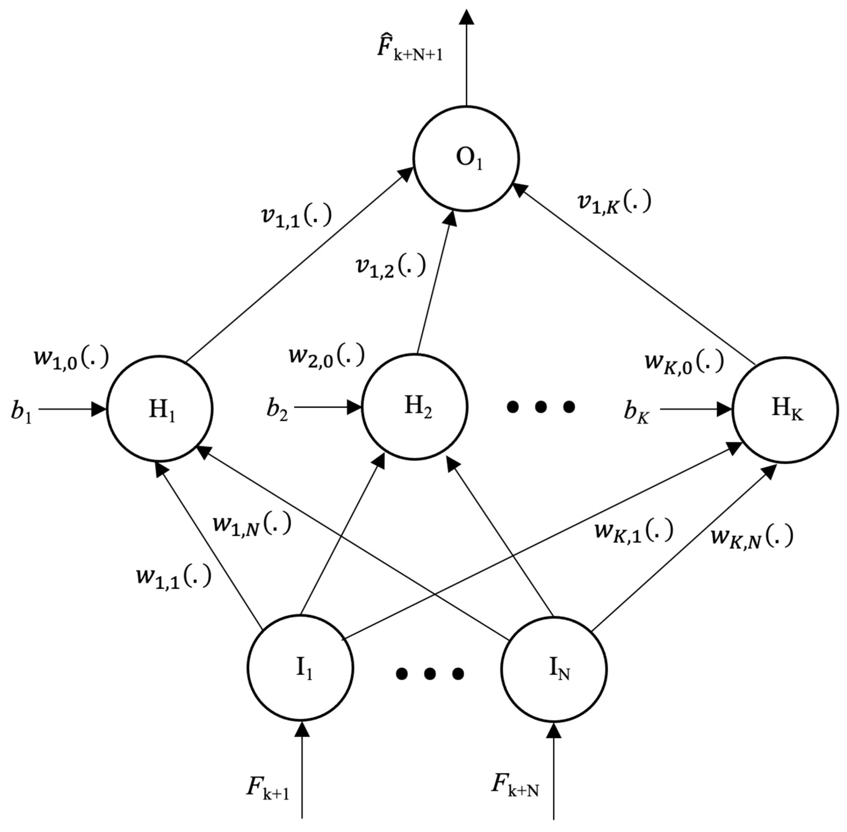
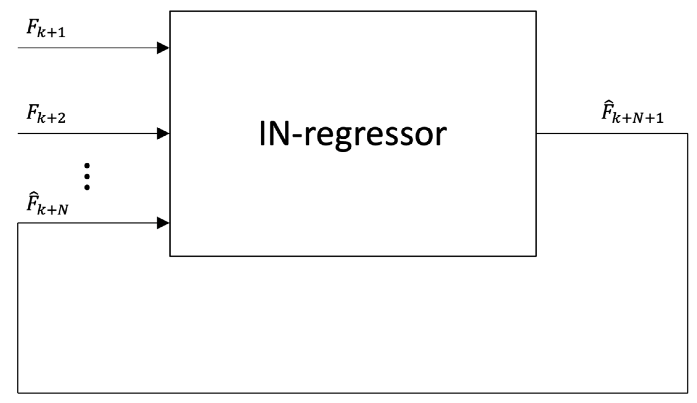
2. An IN-Regressor Parametric Models for Prediction

Figure 1 displays an IN in its two equivalent representations, namely the membership–function–representation in Figure 1a and the interval–representation in Figure 1b. More specifically, the membership–function–representation is identical to a probability distribution function; therefore, it is amenable to interpretations, whereas its equivalent interval-representation lends itself to useful algebraic operations in the context of mathematical lattice theory.

The space of INs is known to be a cone in a linear space. Therefore, linear models such as ARMA models can be developed. The work in [18] has proposed a nonlinear model in the space of INs implemented by three-layer feed-forward neural network, namely IN-based Neural Network or INNN for short, with N = 2 inputs. In this work, the number of inputs of the INNN is increased to N as shown in Figure 2. More specifically, the input to INNN is an N-tuple (F_k+1, …, F_k+N) of INs, where k ∈ {0, …, n − N} and n is the total number of INs in a time-series F₁, …, F_n. The INNN is trained to learn mapping an N-tuple (F_k+1, …, F_k+N) to the true output IN F_k+N+1. In other words, the nonlinear regressor model implemented by the INNN is trained to learn the physical “law” that generates the non-stationary time-series of INs regarding grape maturity. More specifically, a sliding window of size N INs is used at times k∈{0, …, n − N} to generate an N-tuple (F_k+1, …, F_k+N) of INs. We point out that an IN in this work represents a grape image data regarding the maturity of a grape bunch as described in [18].

The architecture in Figure 2 is trained to learn a difference equation that calculates an estimate ${\widehat{F}}_{k+N+1}$ of the true future IN F_k+N+1 based on N past INs F_k+1, …, F_k+N. Learning involves the calculation of a set of parameters that minimize the error between the estimate ${\widehat{F}}_{k+N+1}$ and the true output IN F_k+N+1 induced from a training image. Algorithm 1 describes the training of the INNN based on a genetic algorithm (GA) [18]. In particular, error minimization is pursued by a GA whose cost function is the metric distance between the estimate ${\widehat{F}}_{k+N+1}$ and the true output IN F_k+N+1. The population of chromosomes is a number of parameters including: (a) the set of weights of the neural network, (b) the parameters of the activation function of each neuron and (c) the set of biases for all neurons. In this case, the activation function is a sigmoid.

Algorithm 1. IN-Regressor Training by a Genetic Algorithm (GA)

Consider the training data set. Generate an initial population of parameter sets. for g generations do Evaluate individuals using the distance between the IN-regressor computed output IN (prediction) estimate and the true output IN. Apply the genetic operators. end for

In contrast to the INNN model presented in [18], which used only measured INs as inputs, the IN-regressor model in this paper uses, in addition, previous predictions as inputs to calculate predictions for future days. Figure 3 delineates the operation of the recursive IN-regressor with Ν inputs. In other words, for the calculation of a maturity prediction for a particular day, one or more of the input INs is actually a previous prediction. In this manner, the recursive scheme in Figure 3 tests the capacity of the proposed IN-regressor to learn the physical “law” that generates a time-series of INs regarding grape maturity.

In terms of Computational Intelligence, the proposed IN-regressor model can be interpreted as a multilayer Fuzzy Inference System (FIS) for deep learning. In conclusion, knowledge is induced from the data in the form of rules; furthermore, fuzzy lattice reasoning (FLR) explanations of the IN-regressor answers can be given as demonstrated below.

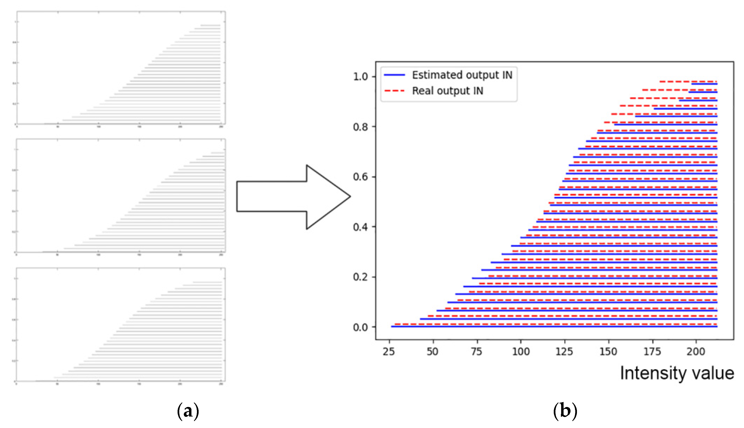
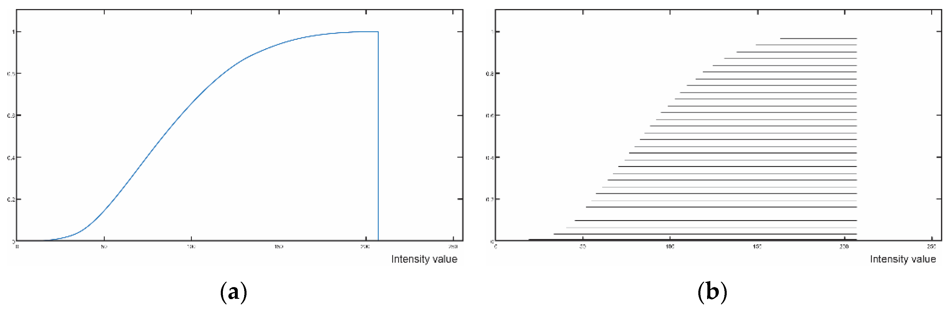
3. Experimental Results

Grape maturity at harvest time is based on the composition balance of several maturity-related chemical compounds and sensory attributes such as color and taste [19]. In order to exploit composition changes and decide on optimal harvest time, it is necessary to perform sensory assessments, i.e., ripeness evaluation, optimally by using non-destructive methods. Toward this end, Red–Green–Blue (RGB) color imaging has been used to calculate the color intensity distribution on grape images while ripening. More specifically, the green channel histogram was represented by an IN [18].

This work extends the IN-regressor in [18] whose results are partly presented below for comparison reasons. More specifically, in [18], only two inputs were used, i.e., N = 2 in Figure 2; whereas, in this work, additional experiments were carried out using both N = 3 and N = 4 in order to study the robustness of the prediction when incrementally more past data were used for prediction. Moreover, in [18], three different training modes were used, namely (a) only One (the first) data sample, (b) Every Other data sample, and (c) nearly the First Half the data samples; whereas, in this work, an additional training mode was used, that is, (d) nearly the First Third of the data samples were also employed for training in order to study the robustness of the prediction when incrementally more data were used to train the IN-regressor. An IN-regressor was trained by the GA in Algorithm 1.

A trained IN-regressor was tested in two different modes, namely “forward” and “recursive” using all the remaining (non-training) data. During “forward” testing, the N-tuple of INs inputs to the IN-regressor included exclusively real (true) INs induced from images, whereas, during “recursive” testing, the N-tuple of INs input to the IN-regressor progressively included ever more of its previous IN predictions as shown in Figure 3. Both “forward” and “recursive” testing were preceded by the same training.

Each different training/testing mode has a particular experimental value as explained in the following. More specifically, One, First Third, and First Half modes use progressively ever more training data; the Every Other mode indicates the effects of reducing the sampling rate by 2, by sampling every other day. Finally, the recursive scheme, in particular, demonstrates an IN-regressor’s capacity to learn the physical “law” that generates the time-series of INs regarding grape maturity toward achieving long-term predictions. In the experiments below, an interval-representation of an IN included L = 32 levels; moreover, the time-series of n = 13 INs in [18] was used.

The results for N = 2 have been detailed in [18].

Table 1. Training/Testing distance error Average and Standard Deviation using N = 3 inputs. The training set included only one sample, i.e., a triplet of INs as input and one output.

Training		Testing
		Forward		Recursive
Data	Error	Data	Error	Data	Error
$\left(F_1,F_2,F_3\right)\to F_4$	0.20
		$\left(F_2,F_3,F_4\right)\to F_5$	8.53	$\left(F_2,F_3,{\widehat{F}}_4\right)\to F_5$	13.05
		$\left(F_3,F_4,F_5\right)\to F_6$	10.68	$\left(F_3,{\widehat{F}}_4,{\widehat{F}}_5\right)\to F_6$	14.97
		$\left(F_4,F_5,F_6\right)\to F_7$	12.40	$\left({\widehat{F}}_4,{\widehat{F}}_5,{\widehat{F}}_6\right)\to F_7$	10.61
		$\left(F_5,F_6,F_7\right)\to F_8$	9.66	$\left({\widehat{F}}_5,{\widehat{F}}_6,{\widehat{F}}_7\right)\to F_8$	12.02
		$\left(F_6,F_7,F_8\right)\to F_9$	13.54	$\left({\widehat{F}}_6,{\widehat{F}}_7,{\widehat{F}}_8\right)\to F_9$	19.87
		$\left(F_7,F_8,F_9\right)\to F_{10}$	15.41	$\left({\widehat{F}}_7,{\widehat{F}}_8,{\widehat{F}}_9\right)\to F_{10}$	27.01
		$\left(F_8,F_9,F_{10}\right)\to F_{11}$	15.00	$\left({\widehat{F}}_8,{\widehat{F}}_9,{\widehat{F}}_{10}\right)\to F_{11}$	30.48
		$\left(F_9,F_{10},F_{11}\right)\to F_{12}$	2.60	$\left({\widehat{F}}_9,{\widehat{F}}_{10},{\widehat{F}}_{11}\right)\to F_{12}$	19.27
		$\left(F_{10},F_{11},F_{12}\right)\to F_{13}$	3.27	$\left({\widehat{F}}_{10},{\widehat{F}}_{11},{\widehat{F}}_{12}\right)\to F_{13}$	21.36
Average	0.20		10.12		18.74
Standard Deviation	0		4.68		6.82

,

Table 2. Training/Testing distance error Average and Standard Deviation using N = 3 inputs. Every Other data sample, i.e., a triplet of INs as input and one output, was used for training.

Training		Testing
		Forward		Recursive
Data	Error	Data	Error	Data	Error
$\left(F_1,F_2,F_3\right)\to F_4$	2.29
		$\left(F_2,F_3,F_4\right)\to F_5$	4.84	$\left(F_2,F_3,{\widehat{F}}_4\right)\to F_5$	5.76
$\left(F_3,F_4,F_5\right)\to F_6$	4.56
		$\left(F_4,F_5,F_6\right)\to F_7$	4.67	$\left(F_4,F_5,{\widehat{F}}_6\right)\to F_7$	6.22
$\left(F_5,F_6,F_7\right)\to F_8$	1.77
		$\left(F_6,F_7,F_8\right)\to F_9$	3.53	$\left(F_6,F_7,{\widehat{F}}_8\right)\to F_9$	23.36
$\left(F_7,F_8,F_9\right)\to F_{10}$	2.87
		$\left(F_8,F_9,F_{10}\right)\to F_{11}$	5.26	$\left(F_8,F_9,{\widehat{F}}_{10}\right)\to F_{11}$	10.02
$\left(F_9,F_{10},F_{11}\right)\to F_{12}$	2.93
		$\left(F_{10},F_{11},F_{12}\right)\to F_{13}$	5.30	$\left(F_{10},F_{11},{\widehat{F}}_{12}\right)\to F_{13}$	3.19
Average	2.89		4.72		9.71
Standard Deviation	1.05		0.71		8.01

,

Table 3. Training/Testing distance error Average and Standard Deviation using N = 3 inputs. The training set included approximately the First Third of the total number of data samples.

Training		Testing
		Forward		Recursive
Data	Error	Data	Error	Data	Error
$\left(F_1,F_2,F_3\right)\to F_4$	2.69
$\left(F_2,F_3,F_4\right)\to F_5$	0.77
$\left(F_3,F_4,F_5\right)\to F_6$	3.62
$\left(F_4,F_5,F_6\right)\to F_7$	1.10
		$\left(F_5,F_6,F_7\right)\to F_8$	4.23	$\left(F_5,F_6,{\widehat{F}}_7\right)\to F_8$	8.12
		$\left(F_6,F_7,F_8\right)\to F_9$	3.97	$\left(F_6,{\widehat{F}}_7,{\widehat{F}}_8\right)\to F_9$	14.48
		$\left(F_7,F_8,F_9\right)\to F_{10}$	5.74	$\left({\widehat{F}}_7,{\widehat{F}}_8,{\widehat{F}}_9\right)\to F_{10}$	20.75
		$\left(F_8,F_9,F_{10}\right)\to F_{11}$	5.73	$\left({\widehat{F}}_8,{\widehat{F}}_9,{\widehat{F}}_{10}\right)\to F_{11}$	24.01
		$\left(F_9,F_{10},F_{11}\right)\to F_{12}$	6.37	$\left({\widehat{F}}_9,{\widehat{F}}_{10},{\widehat{F}}_{11}\right)\to F_{12}$	22.20
		$\left(F_{10},F_{11},F_{12}\right)\to F_{13}$	8.67	$\left({\widehat{F}}_{10},{\widehat{F}}_{11},{\widehat{F}}_{12}\right)\to F_{13}$	22.34
Average	2.05		5.78		18.65
Standard Deviation	1.34		1.69		6.12

and

Table 4. Training/Testing distance error Average and Standard Deviation using N = 3 inputs. The training set included approximately the First Half of the total number of data samples.

Training		Testing
		Forward		Recursive
Data	Error	Data	Error	Data	Error
$\left(F_1,F_2,F_3\right)\to F_4$	3.15
$\left(F_2,F_3,F_4\right)\to F_5$	0.61
$\left(F_3,F_4,F_5\right)\to F_6$	4.71
$\left(F_4,F_5,F_6\right)\to F_7$	1.20
$\left(F_5,F_6,F_7\right)\to F_8$	1.59
		$\left(F_6,F_7,F_8\right)\to F_9$	6.56	$\left(F_6,F_7,{\widehat{F}}_8\right)\to F_9$	6.93
		$\left(F_7,F_8,F_9\right)\to F_{10}$	7.07	$\left(F_7,{\widehat{F}}_8,{\widehat{F}}_9\right)\to F_{10}$	10.15
		$\left(F_8,F_9,F_{10}\right)\to F_{11}$	6.81	$\left({\widehat{F}}_8,{\widehat{F}}_9,{\widehat{F}}_{10}\right)\to F_{11}$	13.90
		$\left(F_9,F_{10},F_{11}\right)\to F_{12}$	8.12	$\left({\widehat{F}}_9,{\widehat{F}}_{10},{\widehat{F}}_{11}\right)\to F_{12}$	11.09
		$\left(F_{10},F_{11},F_{12}\right)\to F_{13}$	3.64	$\left({\widehat{F}}_{10},{\widehat{F}}_{11},{\widehat{F}}_{12}\right)\to F_{13}$	13.06
Average	2.25		6.44		11.03
Standard Deviation	1.66		1.67		2.73

detail the results for N = 3.

Table 5. Training/Testing distance error Average and Standard Deviation (Std) using N ∈ {2,3,4} inputs for four training modes: (1) One sample, (2) Every Other sample, (3) First Third of the samples, and (4) First Half of the samples.

N	Training Mode	Training Error	Testing Error (Average/Std)
		(Average/Std)	Forward	Recursive
2	(1) One sample	0.10/0	11.45/9.17	37.87/9.96
	(2) Every Other sample	3.21/1.26	10.54/8.74	17.85/11.93
	(3) First Third of the samples	5.97/3.28	7.92/3.43	18.54/4.53
	(4) First Half of the samples	5.15/3.79	6.84/4.12	7.57/4.87
3	(1) One sample	0.20/0	10.12/4.68	18.74/6.82
	(2) Every Other sample	2.89/1.05	4.72/0.71	9.71/8.01
	(3) First Third of the samples	2.05/1.34	5.78/1.69	18.65/6.12
	(4) First Half of the samples	2.25/1.66	6.44/1.67	11.03/2.73
4	(1) One sample	0.14/0	14.09/3.68	20.21/8.92
	(2) Every Other sample	1.95/0.48	4.99/1.95	9.64/4.66
	(3) First Third of the samples	0.93/0.32	10.85/4.25	25.89/2.75
	(4) First Half of the samples	1.64/0.99	4.30/0.96	6.65/2.32

summarizes the results for all training/testing modes for all N = 2, N = 3, and N = 4. Table 5 clearly demonstrates that, as N increases, the training error decreases as well as the corresponding standard deviation due to more accurate predictions. A similar observation holds for the testing error, for the same reason, even though the testing error is significantly larger with significantly larger standard deviation. For constant N, as the number of training data increases, so does the error, due to “curve-fitting” problems; nevertheless, often the corresponding standard deviation appears to decrease. However, an IN-regressor demonstrates a good capacity for generalization on the testing data because, for constant N, as the number of training data increases, the error decreases even though it is clearly larger than the corresponding training error. Especially promising is the performance of the IN-regressor in the recursive mode for N = 4 when the First Half of the data were used for training. Then, an average of 6.65 was recorded with a standard deviation of 2.32 recorded compared to 4.30 and 0.96, respectively, recorded in the forward mode. The significance of the latter is that the proposed IN-regressor could potentially make accurate long-term predictions, thus providing time to engage both human labor and equipment for grape harvest.

An N-tuple of INs input to the IN-regressor followed by its corresponding output IN can be interpreted as a fuzzy rule (i.e., knowledge), of a “Mamdani type” FIS, induced from the training data as indicated in Figure 4, where Figure 4a shows the rule’s antecedent and Figure 4b shows the rule’s consequent.

4. Discussion and Conclusions

Agriculture 4.0 [1], including viticulture, calls for intelligent decision-making. Of special interest is the accurate prediction of the grape maturity in order to timely engage both human labor and equipment for harvest. This work has proposed a parametric regressor, namely IN-regressor, model for grape maturity prediction.

The IN-regressor processes Intervals’ Numbers (INs) with the advantage that an IN represents a distribution of data including all-order data statistics. Hence, instead of representing the maturity status of grapes by few numbers, e.g., the mean and standard deviation of a number of measurements, the maturity status of grapes is represented by a distribution of measurements, i.e., all-order data statistics, toward better decision-making. A neural network architecture, namely INNN, with N inputs (INs) and one output (IN) was shown to implement the proposed IN-regressor.

Extensive computational experiment here has demonstrated that an IN-regressor can accurately predict the grape maturity status, especially for larger N as well for more training data. Therefore, the IN-regressor be used for predicting the grape harvest time. Furthermore, especially promising is a recursive IN-regressor scheme for long-term prediction.

The proposed IN-regressor has been interpreted as a deep learning FIS with a capacity to suggest explanations for its answers by “Mamdani type” fuzzy rules.

Technical future work will pursue one (or more) neural network layer(s) in the input as a filter that normalizes the effects of taken a grape image at different azimuth /altitude /distance /lighting conditions, etc. Furthermore, a faster algorithm for optimization will be pursued instead of a GA. An extension of this work can also demonstrate far more experimental results using data already acquired on-the-field.

As grapes mature, their image statistics change with time. Therefore, since an IN represents a distribution of image statistics regarding grape maturity, it follows that a time-series of INs by definition represents a non-stationary time-series process. Hence, the proposed IN-regressor can be used for predicting a future probability distribution function from past probability distribution functions in a non-stationary time-series. Therefore, apart from agriculture, this work has presented potentially useful instruments for other application domains including the environment [20], medicine [21], econometrics [22], stock-market data [23], and other.

References

1. Rose, D.C.; Wheeler, R.; Winter, M.; Lobley, M.; Chivers, C.-A. Agriculture 4.0: Making it work for people, production, and the planet. Land Use Policy 2021, 100, 104933. [Google Scholar] [CrossRef]
2. Sohaib Ali Shah, S.; Zeb, A.; Qureshi, W.S.; Arslan, M.; Ullah Malik, A.; Alasmary, W.; Alanazi, E. Towards fruit maturity estimation using NIR spectroscopy. Infrared Phys. Technol. 2020, 111, 103479. [Google Scholar] [CrossRef]
3. Perry, T.S. Want a Really Hard Machine Learning Problem? Try Agriculture, Says John Deere Labs. Available online: https://spectrum.ieee.org/view-from-the-valley/robotics/artificial-intelligence/want-a-really-hard-machine-learning-problem-try-agriculture-say-john-deere-labs-leaders (accessed on 19 May 2021).
4. Vrochidou, E.; Tziridis, K.; Nikolaou, A.; Kalampokas, T.; Papakostas, G.A.; Pachidis, T.P.; Mamalis, S.; Koundouras, S.; Kaburlasos, V.G. An Autonomous Grape-Harvester Robot: Integrated System Architecture. Electronics 2021, 10, 1056. [Google Scholar] [CrossRef]
5. Mehdizadeh, S. Using AR, MA, and ARMA Time Series Models to Improve the Performance of MARS and KNN Approaches in Monthly Precipitation Modeling under Limited Climatic Data. Water Resour. Manag. 2020, 34, 263–282. [Google Scholar] [CrossRef]
6. Wang, Q.; Li, S.; Li, R.; Ma, M. Forecasting U.S. shale gas monthly production using a hybrid ARIMA and metabolic nonlinear grey model. Energy 2018, 160, 378–387. [Google Scholar] [CrossRef]
7. Tealab, A.; Hefny, H.; Badr, A. Forecasting of nonlinear time series using ANN. Futur. Comput. Inform. J. 2017, 2, 39–47. [Google Scholar] [CrossRef]
8. Raj, J.S.; Ananthi, J.V. Reccurent Neural Networks and Nonlinear Prediction in Support Vector Machines. J. Soft Comput. Paradig. 2019, 2019, 33–40. [Google Scholar] [CrossRef]
9. Tealab, A. Time series forecasting using artificial neural networks methodologies: A systematic review. Futur. Comput. Inform. J. 2018, 3, 334–340. [Google Scholar] [CrossRef]
10. Kaburlasos, V.G. FINs: Lattice Theoretic Tools for Improving Prediction of Sugar Production From Populations of Measurements. IEEE Trans. Syst. Man Cybern. Part B 2004, 34, 1017–1030. [Google Scholar] [CrossRef] [PubMed]
11. Kaburlasos, V.G. The Lattice Computing (LC) Paradigm. In Proceedings of the the 15th International Conference on Concept Lattices and Their Applications CLA, Tallinn, Estonia, 29 June–1 July 2020; pp. 1–8. [Google Scholar]
12. Kaburlasos, V.G.; Papadakis, S.E. Granular self-organizing map (grSOM) for structure identification. Neural Netw. 2006, 19, 623–643. [Google Scholar] [CrossRef] [PubMed]
13. Kaburlasos, V.G.; Kehagias, A. Fuzzy Inference System (FIS) Extensions Based on the Lattice Theory. IEEE Trans. Fuzzy Syst. 2014, 22, 531–546. [Google Scholar] [CrossRef]
14. Kaburlasos, V.G.; Athanasiadis, I.N.; Mitkas, P.A. Fuzzy lattice reasoning (FLR) classifier and its application for ambient ozone estimation. Int. J. Approx. Reason. 2007, 45, 152–188. [Google Scholar] [CrossRef] [Green Version]
15. Kaburlasos, V.G.; Papakostas, G.A. Learning Distributions of Image Features by Interactive Fuzzy Lattice Reasoning in Pattern Recognition Applications. IEEE Comput. Intell. Mag. 2015, 10, 42–51. [Google Scholar] [CrossRef]
16. Kaburlasos, V.G.; Papakostas, G.A.; Pachidis, T.; Athinellis, A. Intervals’ Numbers (INs) interpolation/extrapolation. In Proceedings of the 2013 IEEE International Conference on Fuzzy Systems (FUZZ-IEEE), Hyderabad, India, 7–10 July 2013; pp. 1–8. [Google Scholar]
17. Vrochidou, E.; Lytridis, C.; Bazinas, C.; Papakostas, G.A.; Wagatsuma, H.; Kaburlasos, V.G. Brain Signals Classification Based on Fuzzy Lattice Reasoning. Mathematics 2021, 9, 1063. [Google Scholar] [CrossRef]
18. Kaburlasos, V.G.; Vrochidou, E.; Lytridis, C.; Papakostas, G.A.; Pachidis, T.; Manios, M.; Mamalis, S.; Merou, T.; Koundouras, S.; Theocharis, S.; et al. Toward Big Data Manipulation for Grape Harvest Time Prediction by Intervals’ Numbers Techniques. In Proceedings of the 2020 International Joint Conference on Neural Networks (IJCNN), Glasgow, UK, 19–24 July 2020; pp. 1–6. [Google Scholar]
19. Kangune, K.; Kulkarni, V.; Kosamkar, P. Automated estimation of grape ripeness. Asian J. Converg. Technol. (AJCT) 2019. Available online: https://asianssr.org/index.php/ajct/article/view/792 (accessed on 20 June 2021).
20. Garnot, V.S.F.; Landrieu, L.; Giordano, S.; Chehata, N. Satellite Image Time Series Classification with Pixel-Set Encoders and Temporal Self-Attention. In Proceedings of the IEEE/CVF Conference on Computer Vision and Patern Recognition (CVPR), Seattle, WA, USA, 13–19 June 2020. [Google Scholar]
21. Dupont, G.; Kalinicheva, E.; Sublime, J.; Rossant, F.; Pâques, M. Analyzing Age-Related Macular Degeneration Progression in Patients with Geographic Atrophy Using Joint Autoencoders for Unsupervised Change Detection. J. Imaging 2020, 6, 57. [Google Scholar] [CrossRef]
22. Greene, W.W.H. Econometric Analysis, 7th ed.; Prentice-Hall: Hoboken, NJ, USA, 2012; ISBN 978-0-273-75356-8. [Google Scholar]
23. Barra, S.; Carta, S.M.; Corriga, A.; Podda, A.S.; Recupero, D.R. Deep learning and time series-to-image encoding for financial forecasting. IEEE/CAA J. Autom. Sin. 2020, 7, 683–692. [Google Scholar] [CrossRef]
Figure 1. Two equivalent representations of an IN: (a) The membership–function–representation, which is identical to a probability distribution function, and (b) the interval–representation which lends itself to useful algebraic operations in the context of mathematical lattice theory.
Engproc 05 00012 g001
Figure 2. Given a time-series of n INs samples, an N × K × 1 forward neural network architecture, which operates on INs, can implement the proposed IN-regressor. The output F ^ k + N + 1 at sampling time k + N, where k ∈ {0, …, nN}, is an estimate/prediction of the true IN Fk+N+1 at the next sampling time.
Engproc 05 00012 g002
Figure 3. Given a time-series of n INs samples, a recursive IN-regressor estimates/predicts IN F ^ k + N + 1 at time k + N, where k ∈ {0, …, nN}, based on past IN predictions such as F ^ k + N etc.
Engproc 05 00012 g003
Figure 4. The first three INs (a) the first three INs F1, F2 and F3, from top to bottom, of the considered time-series of Ins; (b) estimated out IN F ^ 4 (shown in solid intervals) computed in the first line of Table 4 versus the real (true) output IN F4 (shown in dashed intervals).
Engproc 05 00012 g004