Abstract
In this paper, we use the time-frequency wavelet estimators to analyze the robustness of Okun’s Law in the European Union across time and within various economic cycles. We extend the Okun’s Law literature as we focus on Europe, directly estimating the time-frequency varying Okun’s coefficient. We observe that Okun’s coefficient in Europe is unstable at short run (infra and annual cycles). The strength of Okun’s Law is time dependent at short run as linkages between growth and unemployment are stronger only during crisis times. Such instability is explained as unemployment predominates growth, leading to a positive coefficient and weaker strength. However, as the frequencies increase, the coefficient is more stable over time and the strength is higher and homogenous over time.
1. Introduction
Okun’s Law [1] established a negative relationship between unemployment rate variations and the output gap. This relationship estimates that 1% variation in the real output from the potential leads to a 0.33% change in the unemployment rate from the natural rate. For the US, Okun’s Law studies estimated that each 1% deviation in real output leads to an unemployment reduction of 0.4% or a heuristic value of 0.5%. Okun’s Law is a pilar of macroeconomics policy tools due to its ability to easily examine unemployment dynamics according to basic economics conditions (crisis time or expansion period).
The stability of the Okun parameter across time is discussed in the literature focusing on macroeconomic aspects explaining, or not, the effect of structural breaks on the Okun’s Law results. Okun’s coefficient can be considered as stable over time for various countries while different values are noted across countries [2,3]. The stability hypothesis of the Okun parameter is also supported [4,5] as no significant differences were found between parameters estimated over different periods (before and after 1984—Great Moderation). However, some studies highlight an unstable Okun parameter value across time [6,7,8,9,10,11]. The unemployment rate seems react more to real output changes during recessions than in expansion periods or subject to structural breaks [10,12,13,14]. Changes in the Okun coefficients have been observed during the Great Moderation [15,16] and in the 2001 recession [17]. The question of the Okun coefficient stability is still debated today; for example, some authors continue to estimate a static parameter to study the relationships [18] or simply use the intuitive value of 0.5 [19].
Recent studies highlight additional weaknesses of Okun’s Law. For instance, the estimation is not conditional on the frequency, here associated to the period of the business cycles [20,21]. Previous literature indicates that the Okun’s Law debate on stability is related to the different kinds of cycles considered in the studies. Then, Okun’s Law can be stable for some cycles (frequencies) while being unstable for others depending on the speed of recovery and the strength of a shock/recession. The output growth volatility transfer from short run cycles (1–4 years) to long run cycles (8–16 years) during the Great Moderation period has been observed [22,23]. These results can explain some variability in Okun’s coefficients across time while supporting the frequency hypothesis. Relevant results were found using time-frequency analysis with a continuous wavelet coherence phase [20]. The Okun coefficient is time-frequency varying but not asymmetric as the value is not dependent on crisis and expansion periods. At the same time, the heuristic value of 0.5% is observed at specific frequencies. Using phase analysis, it has been found that output (and growth) is predominantly variable of the relation. The time-frequency variation of Okun’s coefficient and the output gaps leads on unemployment are also supported [21]. However, few papers have analyzed Okun’s Law in Europe, assuming that results observed for the US are applicable to European situations. But the European business cycles and labor market are different, potentially leading to different results for Europe. Since the 2008–2009 crisis, unemployment has been a persistent and structural issue in many European countries (especially in Mediterranean countries such as France, Spain, and Italy).
Time-frequency analysis is then suitable to study the relationship between variables, particularly the coherence and phase. Multiple studies focus on the application of wavelets in finance to highlight linkages between commodities, stock indices, and financial assets [24,25,26,27,28] to outline risk transmission mechanisms or contagion effects between major stock indices. The notion of wavelet gain is developed [20,29] in order to assess the absolute value of a parameter’s regression model (applied for the Okun framework, among others) and analyze the phase to assess the sign and the lead–lag relationship. In parallel, the concept of wavelet gain is extended by time-frequency estimators [30,31] to directly estimate the beta at each time and frequency with its sign (positive or negative).
In this paper, we use the time-frequency wavelet estimators to analyze Okun’s Law in the European Union. We extend the Okun’s Law literature as we focus on Europe and estimate the time-frequency varying Okun’s coefficient. We first present the technical improvement of wavelet time-frequency estimators, and we then discuss and analyze the results.
2. Materials and Methods
Wavelets are an extension of the spectral analysis of time series, allowing the decomposition of a chronic in the time-frequency space [32,33,34,35,36,37]. We distinguish two forms of wavelet decomposition processes: the discrete process, called maximal overlap discrete wavelets transform (MODWT); and the continuous process, called continuous wavelet transform (CWT). The main difference between MODWT and CWT is the type of wavelets used, the accuracy in the frequency scale, and the computational time. MODWT is based on a dyadic scale decomposition in which frequency components are ranked into wavelet frequency bands of a length equal to a multiple of 2 only. The CWT is finer and can more accurately distinguish between frequencies. In addition, CWT provides cross-transformation of two variables useful to analysis interaction and between them across time and frequencies.
The CWT is based on a wavelet mother serving as a filter to extract information from a time series of length N. This function will be shifted by a time parameter and dilated by s, a frequency scale parameter, generating the wavelet family composed by “wavelet daughters” representing each version of according to and s.
The initial chronic will be projected in the generating the wavelet coefficients, . These coefficients represent the variations in around an area around with a frequential length s.
where is the complex conjugate of .
Then, the CWT of generates multiple sub-chronics of the same length, N, at each frequency scale. The inverse process, called inverse continuous wavelet transform (ICWT), allows the reconstruction of the initial from all of the wavelet coefficients.
The previous equation of ICWT assumes that the expression is non-null and less than . This condition ensures the condition of the existence or admissibility of the wavelet mother [37]:
where is the Fourier transform of the wavelet mother.
This condition indicates and is respected when the wavelet mother is a zero-mean and square norm function, then the variance of is preserved during the process of decomposition and reconstruction. In this paper, we use the complex Morlet wavelet as it provides a good balance between time and frequency representations.
where and , the non-dimensional frequency, equals 6 to satisfy the condition on .
From a CWT based on the Morlet wavelets, we define the notion of wavelet coherence, which is similar to the squared correlation and useful to visualize co-movement between two chronics, and [38]. The two time series are decomposed by CWT providing their respective wavelet coefficients . So, we can compute time-frequency covariance called cross-wavelet decomposition:
is the complex-conjugate of .
The formula of the wavelet coherence, between and is like the R2 one in terms of the ratio of covariance and variance products.
G is a smoothing time-frequency operator.
Time-frequency smoothing is required because the coherence coefficients are complex [39]. The coherence coefficient is between 0 and 1 at each time t and frequency scale s.
The wavelet phase difference (or simply phase) is a complementary notion to the coherence as it contains information on the leadership and sign of the relationship between and . The phase difference function, is the arctangent of the ratio of the imaginary part and real part of the cross-transform :
According to the value of the phase difference between and , we can study the sign and the leadership of the relationship between and as follows:
- -
- : and move together in phase so they are positively correlated. In this case, leads .
- -
- : and move together in anti-phase so they are negatively correlated. In this case, leads .
- -
- and move together in phase so they are positively correlated. In this case, leads .
- -
- : and move together in anti-phase so they are negatively correlated. In this case, leads .
We define the time-frequency estimator as follows:
where is a phase parameter providing the sign of the correlation ([30,31] when chronics are in phase and when chronics are in anti-phase .
We use official data for the European Union quarterly real GDP (Y) and unemployment rate (U) for 2001—Q1 to 2019—Q4. Previously, we computed the GDP growth () and unemployment rate variations to estimate the first difference Okun’s Law equation:
The wavelet coherence indicates the strength (R2) of Okun’s Law while the phase shows which variable leads the relationships. Equation (10) in the time-frequency space is then:
Finally, we apply the time-frequency estimators’ formula (Equation (9)), and we study the time and frequency dynamic of the Okun coefficient.
3. Results and Discussion
Figure 1 shows the coherence, phase difference, and time frequency varying Okun coefficient results. Figure 1a is a 2D presentation of the time-frequency coherence (R2 coefficients) associated with the phase difference represented by arrows. The color code shows the value of the coherence, with red for high coherence and blue for low coherence between the two variables. The direction of the arrows indicates both the sign of the relationship—negative by arrows pointing left and positive by arrows pointing right—and the variable leader. Figure 1b shows a 3D representation of the coherence between the two variables. The analysis of the leader variable is more easily performed from a representation of the phase for a given frequency, which is performed hereafter. The frequency unit is the period related to the cycle. Then, period 2 represents a cycle of 6 months (two quarters), period 4 represents a cycle of 1 year (four quarters), etc.
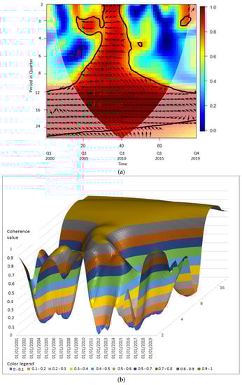
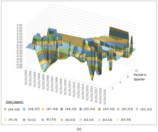
Figure 1.
(a) Two-dimensional representation of wavelet coherence and phase between growth and unemployment rate variations; (b) three-dimensional representation of wavelet coherence; (c) three-dimensional representation of time-frequency varying the Okun coefficient. Corresponding color legends describing coefficents values are put on each figure.
The coherence is strong at high-frequencies between periods 2 and 4 (here, the short-run horizon) only during 2007–2010 (Global Financial Crisis and 2009 Recession). In the long term, for cycles of more than three years, the coherence is very high across time and seems independent of crisis and expansion periods. We can thus conclude that the intensity of the Okun relationship is dependent of the European economic condition (recession expansion) for short cycles (less than 1 year) but remains homogeneous in the longer term. These results are consistent with current literature mainly focused on the US economy as we confirm the frequency hypothesis of Okun’s Law. However, we note that the strength of Okun’s Law is more dependent on short run economics situations, especially crisis times, in Europe than in the US. Then, we notify a frequency asymmetric relation. Okun’s Law is consistent and relevant in the long run but sensitive to economic conditions in the short term.
In addition, the estimation of the Okun coefficient in the time-frequency space extends our interpretation. Figure 1c shows that the Okun coefficient is not stable around the commonly acceptable value of −0.5. Then, the coefficient is more erratic and volatile, especially in the very short term. However, in the long run, the coefficient seems to be more stable as the strength of the relation increases. We also note an unusual result with positive Okun coefficients while a negative one is expected.
In the short term for cycles between 6 months and less than 1 year in length, the coherence is relatively high and the Okun coefficients are decreased and negative from 2001 to Q1 of 2005, reaching its lowest value at −0.9. Growth is the predominant variable, but after 2005 the coefficient is increasing to stabilize around −0.3 until 2010. Here; we note that unemployment leads growth. During the European debt crisis (2011–2012), the Okun coefficient increased to 0 and the coherence sharply decreased to 0. From 2014 to Q1 of 2016, the coherence slowly increases while being non-significant and the Okun coefficient returns to the negative zone at −0.8. Note that unemployment still predominates growth. However, from Q1 of 2016 to mid-2018, the coherence sharply increases and growth leads unemployment, as expected by Okun’s Law. Afterward, we note a positive Okun coefficient with unemployment as the leading variable. For cycles between 1 and 3 years in length, the results show that Okun’s Law is relevant only during crisis times from 2007 to 2012 with growth as the predominant variable. The Okun coefficient is stable at around −0.27. As previously observed, the coherence is non-significant after the debt crisis and sharply decreases as unemployment dominates growth. It seems that when unemployment predominates growth, coherence tends to decrease sharply and the Okun coefficient (usually negative) increases, frequently exceeding zero. For long run cycles with a period above 3 years, we note a stable and negative Okun coefficient around [−0.37, −0.3] with growth as the predominant variable. However, since mid-2015, there has been a slow decline in coherence, a slow increase in the Okun coefficient, and a more frequent predominance of unemployment over growth.
The leadership of unemployment indicates standard unilateral causal representation from growth to unemployment of Okun’s Law is not fully observed, supposing a feedback relationship. This unusual aspect is observed over all business cycles, regardless of the frequencies, and coincides with a decline in the strength of Okun’s Law and its coefficient (turning from negative to positive). The literature mainly focusing on the US economy indicates that this fact is only concentrated on specific frequencies.
We find that, for Europe, the unemployment changes play a greater role especially after the 2008 crash and debt crisis (2011–2012). Consequently, unemployment changes lead over growth, reducing the strength of Okun’s Law, and then tends to affect the coefficient, equating to or exceeding zero more frequently than in the USA. Such results can be explained by the structural unemployment rate being more important in Europe than in the US, for which the labor market is more liquid. Many European countries (for example, France, Spain, and Italy) have suffered high unemployment rate since the 2008–2009 crisis.
4. Conclusions
In this article, we discuss the strength of Okun’s Law for Europe as well as the stability of its coefficient across time and frequencies. We use a wavelet approach distinguishing Okun’s relationship with various economic cycles of different amplitudes. The literature recommends the estimation of the gain in wavelets (the absolute value of the parameter), but our results propose the direct estimation of the time-frequency varying Okun’s coefficient.
We find that the value of Okun’s coefficient and the coherence are then unstable in the short run as unemployment variations more frequently lead growth for infra-annual or annual cycles. However, we assume that the short-run coefficient is relatively stable and negative across time and frequencies in crisis times only (for example, the 2008 crash and debt crisis). In this context, growth is predominant over unemployment, satisfying the Okun’s Law specification. However, when unemployment leads the relation, the coefficient tends to be equal to zero or positive while the coherence declines. This fact is observed for relatively quiet periods or post-crisis periods. We note that the coefficient gradually stabilizes in value as the frequencies increase (i.e., for long-run cycles). For cycles of more than 3 years, the coefficient is stable and insensitive to economic conditions. Okun’s Law is then more relevant for long-run cycle than for short-run cycles in Europe.
Compared with the US, the European Okun’s Law is frequency asymmetric as the coefficient is dependent on crises in the short term but not in the long run. This result is consistent with a previous one indicating that the short-run Okun’s Law is less robust across time than the long-run one. In addition, the standard value of −0.5 is discussed for Europe as the long-run coefficient is close to −0.3, the initial value provided by Okun. This result suggests that the structural unemployment in Europe is stronger and then less affected by economic growth than in the US. This conclusion is also consistent with phase analysis showing a more frequent leadership of unemployment in Europe than commonly observed in the literature for the US.
Funding
This research received no external funding.
Institutional Review Board Statement
Not applicable.
Informed Consent Statement
Not applicable.
Data Availability Statement
The data presented in this study are openly available in the Eurostat database or FRED data website.
Conflicts of Interest
The authors declare no conflict of interest.
References
- Okun, A.M. Potential GNP: Its Measurement and Significance. In Proceedings of the Business and Economic Statistics Section of the American Statistical Association; American Statistical Association: Alexandria, VA, USA, 1962; Volume 7, pp. 98–104. [Google Scholar]
- Galí, J.; Smets, F.; Wouters, R. Slow recoveries: A structural interpretation. J. Money Credit Bank. 2012, 44, 9–30. [Google Scholar] [CrossRef]
- Ball, L.; Leigh, D.; Loungani, P. Okun’s Law: Fit at 50? J. Money Credit Bank. 2017, 49, 1413–1441. [Google Scholar] [CrossRef]
- Fernald, J.G.; Hall, R.E.; Stock, J.H.; Watson, M.W. The Disappointing Recovery of Output after 2009; Working Paper No. w23543; National Bureau of Economic Research: Cambridge, MA, USA, 2017. [Google Scholar]
- Daly, M.C.; Fernald, J.G.; Jordà, O.; Nechio, F. Shocks and Adjustments; Working Paper 2013-32; Federal Reserve Bank of San Francisco: San Francisco, CA, USA, 2017. [Google Scholar]
- Lee, J. The robustness of Okun’s law: Evidence from OECD countries. J. Macroecon. 2000, 22, 331–356. [Google Scholar] [CrossRef]
- Cuaresma, J.C. Okun’s law revisited. Oxf. Bull. Econ. Stat. 2003, 65, 439–451. [Google Scholar] [CrossRef]
- Silvapulle, P.; Moosa, I.A.; Silvapulle, M.J. Asymmetry in Okun’s law. Can. J. Econ. 2004, 37, 353–374. [Google Scholar] [CrossRef]
- Holmes, M.J.; Silverstone, B. Okun’s law, asymmetries and jobless recoveries in the United States: A Markov-switching approach. Econ. Lett. 2006, 92, 293–299. [Google Scholar] [CrossRef]
- Gordon, R.J. Okun’s law and productivity innovations. Am. Econ. Rev. 2010, 100, 11–15. [Google Scholar] [CrossRef]
- Lucchetta, M.; Paradiso, A. Sluggish US employment recovery after the Great Recession: Cyclical or structural factors? Econ. Lett. 2014, 123, 109–112. [Google Scholar] [CrossRef]
- Knotek, E.S., II. How useful is Okun’s law? Econ. Rev.-Fed. Reserve Bank Kans. City 2007, 92, 73–103. [Google Scholar]
- Meyer, B.; Tasci, M. An unstable Okun’s Law, not the best rule of thumb. Fed. Reserve Bank Clevel. Econ. Comment. 2012, 8. [Google Scholar] [CrossRef]
- Grant, A.L. The Great Recession and Okun’s law. Econ. Model. 2018, 69, 291–300. [Google Scholar] [CrossRef]
- Owyang, M.T.; Sekhposyan, T. Okun’s law over the business cycle: Was the great recession all that different? Fed. Reserve Bank St. Louis Rev. 2012, 94, 399–418. [Google Scholar] [CrossRef]
- Valadkhani, A.; Smyth, R. Switching and asymmetric behaviour of the Okun coefficient in the US: Evidence for the 1948–2015 period. Econ. Model. 2015, 50, 281–290. [Google Scholar] [CrossRef]
- Berger, T.; Everaert, G.; Vierke, H. Testing for time variation in an unobserved components model for the US economy. J. Econ. Dyn. Control 2016, 69, 179–208. [Google Scholar] [CrossRef]
- Kamber, G.; Morley, J.; Wong, B. Intuitive and reliable estimates of the output gap from a Beveridge Nelson filter. Rev. Econ. Stat. 2018, 100, 550–566. [Google Scholar] [CrossRef]
- Arai, N. Evaluating the Efficiency of the FOMC’s New Economic Projections. J. Money Credit Bank. 2016, 48, 1019–1049. [Google Scholar] [CrossRef]
- Aguiar-Conraria, L.; Martins, M.; Soares, M.J. Okun’s Law across time and frequencies. J. Econ. Dyn. Control 2020, 116, 103897. [Google Scholar] [CrossRef]
- Krüger, J.; Neugart, M. Dissecting Okun’s law beyond time and frequency. Appl. Econ. Lett. 2021, 28, 1744–1749. [Google Scholar] [CrossRef]
- Crowley, P.M.; Hallett, A.H. Great moderation or “Will o’ the Wisp”? A time-Frequency decomposition of GDP for the US and UK. J. Macroecon. 2015, 44, 82–97. [Google Scholar] [CrossRef]
- Crowley, P.M.; Hallett, A.H. What causes business cycles to elongate, or recessions to intensify? J. Macroecon. 2018, 57, 338–349. [Google Scholar] [CrossRef]
- Aguiar-Conraria, L.; Soares, M.J. The Continuous Wavelet Transform: Moving beyond Uni-and Bivariate Analysis. J. Econ. Surv. 2014, 28, 344–375. [Google Scholar] [CrossRef]
- Bekiros, S.; Nguyen, K.D.; Salah Uddin, G.; Sjo, B. On the time scale behavior of equity-commodity links: Implications for portfolio management. J. Int. Financ. Mark. Inst. Money 2016, 41, 30–46. [Google Scholar] [CrossRef]
- Kahraman, E.; Unal, G. Multiple wavelet coherency analysis and forecasting of metal prices. arXiv 2019, arXiv:1602.01960. [Google Scholar]
- Mestre, R. Stock profiling using time-frequency-varying systematic risk measure. Financ. Innov. 2023, 9, 52. [Google Scholar] [CrossRef]
- Mestre, R. A wavelet approach of investing behaviors and their effects on risk exposures. Financ. Innov. 2021, 7, 24. [Google Scholar] [CrossRef]
- Aguiar-Conraria, L.; Martins, M.; Soares, M.J. Estimating the Taylor Rule in the time-frequency domain. J. Macroecon. 2018, 57, 122–137. [Google Scholar] [CrossRef]
- Mestre, R.; Terraza, M. Time-Frequency varying beta estimation-a continuous wavelets approach. Econ. Bull. 2018, 38, 1796–1810. [Google Scholar]
- Mestre, R.; Terraza, M. Time-frequency varying estimations: Comparison of discrete and continuous wavelets in the market line framework. J. Bank. Financ. Technol. 2019, 3, 97–111. [Google Scholar] [CrossRef]
- Grossmann, A.; Morlet, J. Decomposition of Hardy functions into square integrable wavelets of constant shape. SIAM J. Math. Anal. 1984, 15, 723–736. [Google Scholar] [CrossRef]
- Meyer, Y. Ondelettes et algorithmes concurrents. Actual. Mathématiques Sci. Arts 1990, 7, 217–381. [Google Scholar]
- Mallat, S. A theory for multiresolution signal decomposition: The wavelet representation. IEEE Trans. Pattern Anal. Mach. Intell. 1989, 11, 674–693. [Google Scholar] [CrossRef]
- Mallat, S. A Wavelet Tour of Signal Processing: The Sparce Way, 3rd ed.; AP Professional: London, UK, 2009. [Google Scholar]
- Mallat, S. Une Exploration des Signaux en Ondelettes; Ecole Polytechnique: Paris, France, 2000. [Google Scholar]
- Daubechies, I. Ten Lectures on Wavelets; Conference Series of Applied Mathematics; Society for Industrial and Applied Mathematics: Philadelphia, PA, USA, 1992. [Google Scholar]
- Grinsted, A.; Moore, J.C.; Jevrejeva, S. Application of the cross wavelet transform and wavelet coherence to geophysical time series. Nonlinear Process. Geophys. 2004, 11, 561–566. [Google Scholar] [CrossRef]
- Torrence, C.; Compo, G. A practical guide to wavelet analysis. Bull. Am. Meteorol. Soc. 1998, 79, 61–78. [Google Scholar] [CrossRef]
Disclaimer/Publisher’s Note: The statements, opinions and data contained in all publications are solely those of the individual author(s) and contributor(s) and not of MDPI and/or the editor(s). MDPI and/or the editor(s) disclaim responsibility for any injury to people or property resulting from any ideas, methods, instructions or products referred to in the content. |
© 2023 by the author. Licensee MDPI, Basel, Switzerland. This article is an open access article distributed under the terms and conditions of the Creative Commons Attribution (CC BY) license (https://creativecommons.org/licenses/by/4.0/).