Abstract
El Niño-Southern Oscillation (ENSO) is caused by periodic fluctuations in sea surface temperature and overlying air pressure across the Equatorial Pacific region. ENSO has a global impact on weather patterns and can cause severe weather events, such as heat waves, floods, and droughts, affecting regions far beyond the tropics. Therefore, forecasting ENSO with longer lead times is of great importance. This study utilizes Long Short-Term Memory (LSTM) network to predict ENSO events in the coming year based on environmental variables from previous years, including sea-surface temperature, sea level pressure, zonal wind, meridional wind, and zonal wind flux. These environmental variables are collected only inside certain spatial and temporal windows and used to forecast ENSO events. Furthermore, this study investigates how the size of these spatial and temporal windows influences the generalization accuracy of forecasting ENSO events. The size of spatial and temporal windows is optimized based on the generalization accuracy of the LSTM network in forecasting ENSO events. Our results indicated that the accuracy of the ENSO forecast is significantly sensitive to the extent of spatial and temporal windows. Specifically, increasing the temporal window size from one to nine years and the spatial window from 0 to 17.7 geographical degrees resulted in generalization accuracies, ranging from 40.1% to 83% in forecasting Central Pacific ENSO and 39.2% to 65% in forecasting Eastern Pacific ENSO.
1. Introduction
El Niño-Southern Oscillation (ENSO) refers to the cyclic variations in sea-surface temperature (SST) and air pressure in the overlying atmosphere in the Equatorial Pacific Ocean. It has two phases—El Niño and La Niña—characterized by warm and cold conditions. El Niño events bring above-average SST in the central and east-central Equatorial Pacific. These conditions typically result in warmer temperatures over the western and northern United States and wetter than average conditions over the US Gulf Coast and Florida during winter. Conversely, La Niña events cause below-average SST in the east-central Equatorial Pacific. During La Niña, winter temperatures are warmer in the southeast and colder than average in the northwestern regions of the United States. Approximately every four years, the SST of the tropical Pacific becomes exceedingly warm, leading to abnormal global climate patterns [1].
The National Oceanic and Atmospheric Administration (NOAA) uses the Oceanic Niño Index (ONI) to identify ENSO events. ONI determines ENSO events by averaging the SST anomalies for three consecutive months in the Niño 3.4 region (5° S–5° N, 170° W–120° W). An ONI greater than 0.5 °C for five consecutive months indicates El Niño, while an ONI less than −0.5 °C for five consecutive months indicates La Niña. Studies have shown that ENSO events concentrated in the Central Pacific (CP) and Eastern Pacific (EP) regions differ, not only in the SST anomaly patterns but also in the oceanic surface currents and their impact on the global climate [2,3].
EP El Niño has a larger SST anomaly centered at 120° W than CP El Niño (also known as El Niño Modoki). In contrast, CP El Niño has a weaker SST anomaly and tends to shift westwards (150° W) during its mature phase [4]. EP La Niña and CP La Niña show differences in the physical mechanism of SST anomaly development [5,6], tropical climate responses, and global environmental impact [2]. Forecasting the type of ENSO events could help prepare for their global repercussions.
State-of-the-art research has applied both dynamical and statistical models to forecast ENSO events. Dynamical models utilize physical laws to conserve the ocean, land, and atmosphere and their interactions to predict ENSO events, while statistical models rely on statistical learning patterns from historical data [7]. While dynamical models require scientists to develop specific mathematical and physical laws to model the relationship between different parameters and ENSO events, statistical models learn those relationships automatically from historical data. The downside is that statistical models, especially deep learning models, do not provide a clear and easy-to-understand mathematical representation of the patterns they have learned. A Long Short-Term Memory (LSTM) network is a recurrent neural network (RNN) tailored for sequential prediction problems with the help of memory gates. This study applies the LSTM network for forecasting ENSO events, given its proven capability in effectively capturing the non-linear complexities of multi-variate time series [8,9,10].
The first step of this study is to optimize the size of spatial and temporal windows, where environmental features related to forecasting ENSO events are extracted. The environmental features include SST, sea level pressure (SLP), zonal wind (ZW), meridional wind (MW), and zonal wind flux (WF). Next, the environmental features, extracted from varying spatial and temporal window sizes, are fed to an LSTM network to forecast ENSO events in the next year to determine which window size results in the highest generalization accuracy. It was shown that the generalization accuracy significantly depends on the spatial and temporal window sizes.
The remainder of this paper is organized as follows. Section 2 reviews select literature in ENSO forecasting. Section 3 describes the data collection and preprocessing. Section 4 outlines the methodology to optimize the size of spatial and temporal windows, and Section 5 discusses the experimental results. Section 6 concludes the paper with a summary of findings and future directions.
2. Literature Review
While ENSO events have been forecasted using statistical [11,12,13] and dynamical models [14,15] in the literature, this section focuses on reviewing statistical methods since our proposed model is also statistical.
Early studies utilized Artificial Neural Networks (ANNs) with the leading empirical orthogonal functions of wind stress or SLP as input [16]. These studies yielded a correlation coefficient (CC) of 0.6 for the prediction period of 1980–1990 and 0.1 for 1950–1970. Baawain et al. [17] used a multi-layer perceptron to predict ENSO events with a one-year lead time. Ham et al. [18] employed transfer learning to train a Convolutional Neural Network (CNN) on both Coupled Model Intercomparison Project Phase 5 (CMIP5) data and reanalysis data for the training period (1871–1973). Their results showed that the correlation coefficient (CC) of the observed and forecasted Niño 3.4 index is above 0.5 for a lead time of 17 months. Martínez-Alvarado et al. [19] used Support Vector Regressor (SVR) and Bayesian neural networks to forecast the tropical SST anomalies for a lead time of up to 15 months. The results demonstrated that the Bayesian neural network model outperformed the SVR. Noteboom et al. [20] proposed a hybrid model using autoregressive integrated moving average and ANN to predict ENSO events with a one-year lead time. Guo et al. [21] proposed a hybrid neural network model that combines ensemble empirical mode decomposition with a CNN and LSTM network. Finally, Peter et al. [22] attempted to forecast ENSO events using Gaussian density neural networks and quantile regression neural network ensembles. These models can assess the predictive uncertainty of the forecast by predicting a Gaussian distribution and the quantiles of the forecasts, respectively.
Several studies have explored the effectiveness of combining statistical and dynamical models for forecasting ENSO events. Hong et al. [23] developed a dynamical-statistical forecast model for predicting SST anomalies, which achieved a CC of 0.8 for a lead time of 12 months. Meanwhile, Zhang et al. [24] used Bayesian model averaging (BMA) to combine the results of three statistical and one dynamical model to forecast ONI. They applied an expectation-maximization algorithm to derive the maximum likelihood estimation for model parameters. Their combined statistical–dynamical model outperformed either statistical or dynamical models when used alone. Finally, Ha et al. [25] proposed an encoder–decoder structure for predicting river flow using ENSO. They achieved an R2 of 0.8 with the CLSTM encoder–decoder and an LSTM network in forecasting Yangtze River flow.
Although not specifically in forecasting ENSO events, the significance of location and time in predicting and forecasting geographical phenomena has been underscored in the literature both theoretically [26,27] and experimentally [28,29]. Here we aim to explore how the extent of spatial and temporal windows, where the environmental features for forecasting ENSO events are extracted, influences the generalization accuracy of an LSTM network.
3. Data Description
Our data consists of seven environmental variables: SST, SLP, ZW, MW, WF, CP’s ONI, and EP’s ONI, recorded at 4697 geographical locations (Figure 1) between 1949 and 2014. These variables were obtained from the following sources:
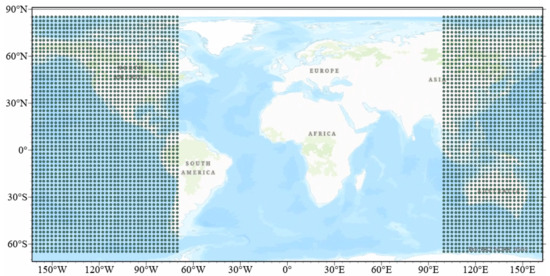
Figure 1.
Data points are separated by 2.5° across latitude and longitude.
- SST data in ℃ was retrieved from NOAA extended reconstructed SST version 3b. The spatial resolution is 1° × 1°. Since this resolution differs from other variables, we used geographical interpolation to convert it to a 2.5° × 2.5° resolution, consistent with the rest of the variables. Additionally, 25% of SST values are missing in this dataset. Therefore, we replaced the missing values of SST with the mean value across the entire region, which is zero.
- SLP in Hecto Pascals was obtained from National Centre for Environmental Climate Prediction (NCEP) reanalysis version 1 [30]. The spatial resolution is 2.5° × 2.5°.
- The horizontal (ZW) and vertical wind (MW) components at 10m depth were obtained from NCEP reanalysis version 1. The spatial resolution is 2.5° × 2.5°.
- The horizontal wind flux (WF) was obtained from NCEP reanalysis version 1. The spatial resolution is 2.5° × 2.5°.
- Details on calculating CP and EP indices from Niño indices are available in [31].
The environmental variables in the dataset represent the three-month averages over December, January, and February. For instance, the SLP data referring to the time 1949-01-01 in the dataset is the average of SLP over December 1948, January 1949, and February 1949.
The continuous values of CP’s ONI and EP’s ONI are transformed into three categories, El Niño where ONI is greater than +0.5, La Niña where ONI is less than −0.5, and Neutral where ONI is between −0.5 and +0.5. There are 24 neutral, 22 El Niño, and 20 La Niña events that occurred in CP, and 34 neutral, 18 La Niña, and 14 El Niño events that occurred in EP between 1949 and 2014. We aim to forecast the ONI class in the next year based on SST, SLP, ZW, MW, and WF from previous years, making this a three-way classification problem.
Feature standardization is a prerequisite for machine learning and deep learning models. Therefore, all variables are standardized to have a zero mean and unit variance.
4. Methodology
An important property of spatial–temporal phenomena is that samples are not independent but rather spatially and temporally auto-correlated. Spatial (temporal) autocorrelation refers to the phenomenon where samples recorded at nearby locations (time) display similar patterns to those recorded further apart. As a result, careful consideration should be given to the spatial–temporal autocorrelation among observations when designing a prediction model.
Every spatial–temporal observation () contains the values of a set of variables at a specific location (s) and time (t). Therefore, a spatial–temporal dataset contains recorded values of features at different locations and times. We define spatial–temporal forecast here as predicting the value of a variable at time t and location s based on the variable’s value and other contributing variables at different locations and previous time stamps. The question we are posing is at what locations (how far from the point where the forecast is being made) and at how many previous timestamps the values of those variables would positively contribute to forecasting the target variable. We refer to the size of the geographical neighborhood as the spatial window size and the number of time stamps going back as the temporal window size. We will measure the forecast generalization accuracy at varying spatial and temporal window sizes. The optimal window sizes are those resulting in the highest generalization accuracy.
4.1. Temporal Window
A temporal window is the number of previous timesteps the environment variable’s values would contribute to forecasting the target variable. For example, a temporal window of one year means environmental variables, SST, SLP, ZW, MW, and WF, recorded from one year ago are used to forecast the occurrence of El Niño, La Niña, or a neutral event in the current year. Similarly, a temporal window of two years means environmental variables recorded from the past two years are used to forecast the occurrence of El Niño, La Niña, or a neutral event in the current year. Figure 2 illustrates the use of a two-year temporal window for forecasting ENSO events. The temporal window size is optimized based on the generalization accuracy of the LSTM network in forecasting ENSO events.
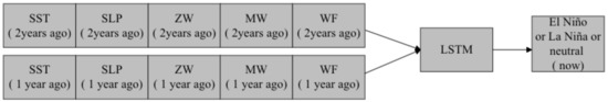
Figure 2.
A temporal window with a size of two years.
4.2. Spatial Window
A spatial window is a distance in geographical degrees from the point where the forecast is being made. The values of the environmental variables that fall within the spatial window would contribute to forecasting the target variable. The spatial window size varies from one point to a circle of radius , where = 3.54 geographical degrees. The coefficient n is treated as a hyperparameter and optimized during training. For example, when the spatial window size is zero, the values of environmental variables SST, SLP, ZW, MW, and WF, recorded only at the forecast point (Figure 3a), are used for forecasting ENSO events in the following year. On the other hand, if the spatial window size is r, the values of those variables recorded at the forecast point and within a distance of 3.54 geographical degrees (Figure 3b) are employed for forecasting ENSO events in the following year. Similarly, a spatial window of size encompasses the values of the environmental variables recorded at the forecasting point and within the distance of 7.08 geographical degrees (Figure 3c) for forecasting ENSO events in the following year.
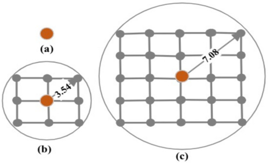
Figure 3.
Varying spatial window sizes: (a) spatial window is one point, (b) spatial window is a circle with a radius of 3.54 = geographical degrees, and (c) spatial window is a circle with a radius of 7.08 geographical degrees.
4.3. LSTM
LSTM overcomes the limitations of traditional RNNs in capturing long-term temporal dependencies in sequential data. Unlike standard RNN, which suffers from the vanishing gradient problem, LSTM uses a gating mechanism to regulate the flow of information through the network. The main component of an LSTM unit is the memory cell, which serves as a storage unit to retain information for longer durations. The memory cell has three gates, input, forget, and output. These gates regulate the flow of information into and outside of the cell, allowing the LSTM to retain or discard information. The input gate decides how much information should be added to the memory cell, while the forget gate decides what information to discard from the memory cell. The output gate regulates the amount of information to be outputted from the memory cell to the next time step or the final prediction. This gating mechanism allows LSTM to capture long-term temporal dependencies from the sequential data. The mathematical equations for information flow in LSTM are given in [32].
The LSTM network consists of an input layer, an LSTM layer, and an output layer. The LSTM layer consists of 32 memory units, ReLU activation, and a dropout of 0.2. Dropout [33] is used as regularization to drop a fraction of randomly selected memory units in the LSTM layer. This means that the information passing through these units is not considered in the forward pass and is not updated during backpropagation, allowing the network to learn robust and generalized data representations. The output layer is a fully connected dense layer with three units, where each unit represents each class. SoftMax is the activation function used in the output layer to generate the probability of each class, and the class with the highest probability is chosen as the target class. The loss function employed in the LSTM network is categorical cross-entropy, and the network is optimized using Adam with a learning rate of 0.001. The model is trained for 100 epochs, and an early stopping algorithm [34] is implemented if the validation loss does not improve for 10 epochs. The network parameters of LSTM are determined by hyperparameter tuning. Notably, adding more LSTM layers to the network led to overfitting.
4.4. Benchmark Models and Evaluation Metrics
To evaluate the performance of the LSTM, we employ Multi-Layer Perceptron (MLP), Random Forest (RF), and CLSTM encoder–LSTM decoder [25] as baselines. The MLP consists of an input layer, two fully connected hidden layers, and an output layer. Two hidden layers comprise 100 units each and ReLU activation. The output layer has three units representing three classes. SoftMax is the activation used in the output layer to generate a probability for each class, and the class with the highest probability is selected as the target class. The loss function employed in the MLP is categorical cross-entropy, and the network is optimized using Adam with a learning rate of 0.001. The model is trained for 100 epochs, and early stopping is implemented if the validation loss does not improve for 10 epochs. The maximum number of features required for splitting in the RF varies with the spatial window size. The number of trees in the RF is 50. We followed the same architecture shown in [25] for the CLSTM encoder–LSTM decoder.
We split the data into 80% for training and 20% for testing. Five-fold cross-validation is implemented on the training dataset to determine the optimal spatial and temporal window sizes and for hyperparameter tuning.
All experiments are evaluated using the F1 score, which measures the model’s accuracy on a dataset. F1 score is the harmonic mean of precision and recall and is calculated as follows. F1 score reaches its best value at one and worst value at zero. The best value for the F1 score is achieved for perfect precision (100%) and recall (100%).
Here, , , , and denotes true positives, true negatives, false positives, and false negatives for class and M denotes the number of classes. True positives and true negatives are the test samples that are correctly classified, and false positives and false negatives are the test samples that LSTM wrongly classifies.
5. Results and Discussions
Figure 4 and Figure 5 present the results of five-fold cross-validation accuracies, expressed as percentages of F1 scores, for predicting ENSO events in CP and EP regions, respectively. Figure 4 indicates that increasing the temporal window from 1 year to 9 years results in an improvement in accuracy of approximately 50%, with the highest accuracy observed at 7 years. Similarly, when varying the spatial window from 0 to , the accuracy increases until and decreases from to . The combination of spatial window size at (7.08 geographical degrees) and temporal window size of 7 years yields the highest cross-validation accuracy and, therefore, is optimal.
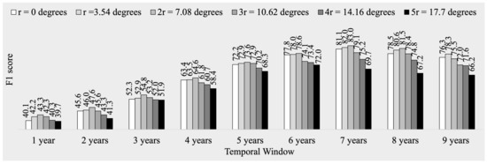
Figure 4.
Five-fold cross validation accuracy (F1 score) in forecasting El Niño and La Niña in CP using LSTM for various spatial and temporal window sizes (values shown in percentage).
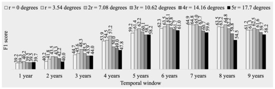
Figure 5.
Five-fold cross validation accuracy (F1 score) in forecasting El Niño and La Niña in EP using LSTM for various spatial and temporal window sizes (values shown in percentage).
For the EP region, the five-fold cross-validation accuracy improves as the temporal window increases from 1 year to 7 years, as depicted in Figure 5. However, when the temporal window is increased from 7 years to 9 years, the accuracy declines. Similarly, regardless of the temporal window size, an increase in the spatial window size from 0 to leads to a rise in accuracy until and a drop in accuracy from to . The optimal spatial and temporal window sizes for the EP region are the same as those for the CP region, a spatial window size of (7.08 geographical degrees) and a temporal window size of 7 years, respectively.
The performance of different models in forecasting ENSO events for a one-year lead time is compared in Table 1. The results indicate that LSTM performs better than the other three baseline models, achieving F1 scores of 0.83 and 0.65 for the CP and EP regions, respectively. The second best-performing models are the CLSTM encoder–LSTM decoder and RF, which exhibit similar accuracies for both regions. The inferior performance of the CLSTM encoder–decoder LSTM model, when compared to LSTM, can be attributed to the flattening of the encoder output, resulting in the loss of spatial structure in environmental variables and their temporal relationships with ENSO events. On the other hand, the limitations of RF lie in its inability to capture the temporal dependencies between environmental variables and ENSO. The MLP performs poorly compared to other models, as it cannot handle the spatial and temporal relationships between environmental variables and ENSO. In summary, LSTM, with optimized spatial and temporal windows, demonstrates its superiority over other baseline models. Specifically, LSTM outperforms RF and CLSTM encoder–decoder LSTM by 1.3 and 1.08 times, respectively, in forecasting ENSO events in the CP and EP regions.

Table 1.
Comparison of different models in forecasting ENSO events (measured in terms of F1 score).
Table 2 presents the precision, recall, and F1 scores for each type of ENSO event, providing insight into the performance of LSTM. Higher precision indicates that the classifier misclassified fewer negative samples as positive samples, and a higher recall indicates that the classifier misclassified fewer positive samples as negative samples. Notably, the recall values for ENSO events in both CP and EP exceed the precision values, indicating that LSTM is suitable for ENSO event forecasting. Further investigation reveals that most misclassified ENSO events have ONI values close to ±0.5.
Table 2.
Highest accuracies in forecasting El Niño and La Niña in CP and EP using LSTM with spatial window of 7.08 geographical degrees and temporal window of 7 years.
Additionally, the proposed model successfully identifies one of the strongest El Niño events from 1997 to 1998. It is worth mentioning that the F1 score of LSTM for EP is slightly reduced compared to CP due to the high-class imbalance ratio, which was not addressed in this study. The experimental results highlight that varying spatial and temporal window sizes, ranging from 0 to 17.7 degrees and 1 year to 9 years, yield forecasting accuracy ranging from 40.1% to 83% for CP and from 39.2% to 65% for EP regions.
6. Conclusions and Future Directions
Our findings demonstrated that the accuracy of forecasting CP (or EP) ENSO events in the coming year could be improved by up to 40% (or 25%) by optimizing the spatial and temporal extent of the environmental variables (i.e., SST, SLP, ZW, MW, and WF) which are used as features in deep learning. Furthermore, it was shown that these optimal spatial and temporal window sizes are 7.08 geographical degrees and 7 years. In our future work, we explore the impact of including additional climate features, such as warm water volume and upper ocean heat content, on the ENSO forecast accuracy of an LSTM. We will also focus on integrating dynamic models into deep learning and studying their impact on forecast accuracies.
Author Contributions
Conceptualization, J.J. and M.H.; methodology, M.H.; formal analysis, J.J. and M.H.; writing—original draft preparation, J.J.; writing—review and editing, J.J. and M.H.; visualization, J.J. and M.H.; supervision, M.H.; project administration, J.J. All authors have read and agreed to the published version of the manuscript.
Funding
This research received no external funding.
Institutional Review Board Statement
Not applicable.
Informed Consent Statement
Not applicable.
Data Availability Statement
The data presented in this study are openly available in GitHub at https://github.com/jahnavijo/ENSO-Dataset.git.
Conflicts of Interest
The authors declare no conflict of interest.
References
- Philander, S. El Niño Southern Oscillation phenomena. Nature 1983, 302, 295–301. [Google Scholar] [CrossRef]
- Hsun-Ying, K.; Jin-Yi, Y. Contrasting Eastern-Pacific and Central-Pacific Types of ENSO. J. Clim. 2009, 22, 615–632. [Google Scholar]
- Jin-Yi, Y.; Tae, K.S. Identifying the types of major El Niño events since 1870. Int. J. Climatol. 2013, 33, 2105–2112. [Google Scholar]
- Mingcheng, C.; Tim, L. ENSO evolution asymmetry: EP versus CP El Niño. Clim. Dyn. 2021, 56, 3569–3579. [Google Scholar]
- Ashok, K.; Behera, S.K.; Rao, S.A.; Weng, H.; Yamagata, T. El Niño Modoki and its possible teleconnection. J. Geo Phys. Lett. 2007, 112. [Google Scholar] [CrossRef]
- Yuan, Y.; Song, Y. Impacts of Different Types of El Niño on the East Asian Climate: Focus on ENSO Cycles. J. Clim. 2012, 25, 7702–7722. [Google Scholar] [CrossRef]
- Barnston Anthony, G.; Tippett Michael, K.; L’Heureux Michelle, L.; Li, S.; DeWitt David, G. Skill of Real-Time Seasonal ENSO Model Predictions during 2002–11: Is Our Capability Increasing? Bull. Am. Meteorol. Soc. 2012, 93, 631–651. [Google Scholar] [CrossRef]
- Qianlong, W.; Yifan, G.; Lixing, Y.; Pan, L. Earthquake Prediction Based on Spatio-Temporal Data Mining: An LSTM Network Approach. IEEE Trans. Emerg. Top. Comput. 2020, 8, 148–158. [Google Scholar]
- Jahnavi, J.; Hashemi, M. Forecasting Atmospheric Visibility Using Auto Regressive Recurrent Neural Network. In Proceedings of the 2020 IEEE 21st International Conference on Information Reuse and Integration for Data Science (IRI), Las Vegas, NV, USA, 11–13 August 2020. [Google Scholar]
- Jahnavi, J.; Hashemi, M. Feature Selection and Spatial-Temporal Forecast of Oceanic Nino Index Using Deep Learning. Int. J. Softw. Eng. Knowl. Eng. 2022, 32, 91–107. [Google Scholar]
- David, C.; Cane Mark, A.; Naomi, H.; Eun, L.D.; Chen, C. A Vector Auto regressive ENSO Prediction Model. J. Clim. 2015, 28, 8511–8520. [Google Scholar]
- Ren, H.L.; Zuo, J.; Deng, Y. Statistical predictability of Niño indices for two types of ENSO. Clim. Dyn. 2018, 52, 5361–5382. [Google Scholar] [CrossRef]
- Hashemi, M. Forecasting El Niño and La Niña Using Spatially and Temporally Structured Predictors and A Convolutional Neural Network. IEEE J. Sel. Top. Appl. Earth Obs. Remote Sens. 2021, 14, 3438–3446. [Google Scholar] [CrossRef]
- Ren, H.L.; Scaife, A.A.; Dunstone, N.; Tian, B.; Liu, Y.; Ineson, S.; Lee, J.Y.; Smith, D.; Liu, C.; Thompson, V.; et al. Seasonal predictability of winter ENSO types in operational dynamical model predictions. Clim. Dyn. 2018, 52, 3869–3890. [Google Scholar] [CrossRef]
- Larson, S.M.; Kirtman, B.P. Drivers of coupled model ENSO error dynamics and the spring predictability barrier. Clim. Dyn. 2017, 48, 3631–3644. [Google Scholar] [CrossRef]
- Tangang, F.T.; Hsieh, W.W.; Benyang, T. Forecasting regional sea surface temperatures in the tropical Pacific by neural network models, with wind stress and sea level pressure as predictors. J. Geophys. Res. Ocean. 1998, 103, 7511–7522. [Google Scholar] [CrossRef]
- Baawain, M.S.; Nour, M.H.; El-Din, A.G.; El-Din, M.G. El Niño southern-oscillation prediction using southern oscillation index and Niño3 as onset indicators: Application of artificial neural networks. J. Environ. Eng. Sci. 2005, 4, 113–121. [Google Scholar] [CrossRef]
- Ham, Y.-G.; Kim, J.-H.; Luo, J.-J. Deep learning for multi-year ENSO forecasts. Nature 2019, 573, 568–572. [Google Scholar] [CrossRef]
- Aguilar-Martinez, S.; Hsieh, W.W. Forecasts of Tropical Pacific Sea Surface Temperatures by Neural Networks and Support Vector Regression. Int. J. Oceanogr. 2009, 2009, 167239. [Google Scholar] [CrossRef]
- Nooteboom, P.D.; Feng, Q.Y.; López Cristóbal, H.-G.E.; Dijkstra Henk, A. Using Network Theory and Machine Learning to predict El Nino. Phys.-Atmos. Ocean. Phys. 2018, 9, 969–983. [Google Scholar] [CrossRef]
- Guo, Y.; Cao, X.; Liu, B.; Peng, K. El Niño Index Prediction Using Deep Learning with Ensemble Empirical Mode Decomposition. Symmetry 2020, 12, 893. [Google Scholar] [CrossRef]
- Petersik, P.J.; Dijkstra, H.A. Probabilistic Forecasting of El Niño Using Neural Network Models. Geophys. Res. Lett. 2020, 47, e2019GL086423. [Google Scholar] [CrossRef]
- Hong, M.; Chen, X.; Zhang, R.; Wang, D.; Shen, S.; Singh, V.P. Forecasting experiments of a dynamical–statistical model of the sea surface temperature anomaly field based on the improved self-memorization principle. Ocean. Sci. 2018, 14, 301–320. [Google Scholar] [CrossRef]
- Zhang, H.; Chu, P.S.; He, L.; Unger, D. Improving the CPC’s ENSO Forecasts using Bayesian model averaging. Clim. Dyn. 2019, 53, 3373–3385. [Google Scholar] [CrossRef]
- Ha, S.; Liu, D.; Mu, L. Prediction of Yangtze River stream flow based on deep learning neural network with El Niño-Southern Oscillation. Sci. Rep. 2021, 11, 11738. [Google Scholar] [CrossRef]
- Hashemi, M.; Karimi, H. Weighted machine learning. Stat. Optim. Inf. Comput. 2018, 6, 497–525. [Google Scholar] [CrossRef]
- Hashemi, M.; Karimi, H.A. Weighted machine learning for spatial-temporal data. IEEE J. Sel. Top. Appl. Earth Obs. Remote Sens. 2020, 13, 3066–3082. [Google Scholar] [CrossRef]
- Hashemi, M.; Alesheikh, A.A.; Zolfaghari, M.R. A spatio-temporal model for probabilistic seismic hazard zonation of Tehran. Comput. Geosci. 2013, 58, 8–18. [Google Scholar] [CrossRef]
- Hashemi, M.; Alesheikh, A.A.; Zolfaghari, M.R. A GIS-based time-dependent seismic source modeling of Northern Iran. Earthq. Eng. Eng. Vib. 2017, 16, 33–45. [Google Scholar] [CrossRef]
- Saha, S.; Moorthi, S.; Wu, X.; Wang, J.; Nadiga, S.; Tripp, P.; Behringer, D.; Hou, Y.T.; Chuang, H.Y.; Iredell, M.; et al. The NCEP Climate Forecast System version 2. J. Clim. 2014, 27, 2185–2208. [Google Scholar] [CrossRef]
- Vimont, D.J.; Alexander, M.A.; Newman, M. Optimal growth of central and east Pacific ENSO events. Geophys. Res. Lett. 2014, 41, 4027–4034. [Google Scholar] [CrossRef]
- Hochreiter Sepp and Schmidhuber Jürgen. Long short-term memory. Neural Comput. 1997, 9, 1735–1780. [Google Scholar] [CrossRef] [PubMed]
- Srivastava, N.; Hinton, G.; Krizhevsky, A.; Sutskever, I.; Salakhutdinov, R. Dropout: A simple way to prevent neural networks from overfitting. J. Mach. Learn. Res. 2014, 15, 1929–1958. [Google Scholar]
- Lutz, P. Early Stopping—However, When. In Neural Networks: Tricks of the Trade, 2nd ed.; Springer: Berlin/Heidelberg, Germany, 2012; pp. 53–67. [Google Scholar]


Disclaimer/Publisher’s Note: The statements, opinions and data contained in all publications are solely those of the individual author(s) and contributor(s) and not of MDPI and/or the editor(s). MDPI and/or the editor(s) disclaim responsibility for any injury to people or property resulting from any ideas, methods, instructions or products referred to in the content. |
© 2023 by the authors. Licensee MDPI, Basel, Switzerland. This article is an open access article distributed under the terms and conditions of the Creative Commons Attribution (CC BY) license (https://creativecommons.org/licenses/by/4.0/).