Abstract
This paper presents a neural network model to estimate arterial blood pressure (ABP) waveforms using electrocardiogram (ECG) and photoplethysmography (PPG) signals and its first two order mathematical derivatives (PPG, PPG). In order to achieve this objective, a lightweight and optimized neural network architecture has been proposed, made of Conv1D and BiLSTM layers. To train the network, the UCI Database “Cuff-Less Blood Pressure Estimation Data Set” has been used, which contains ECG and PPG signals together with the corresponding ABP waveform data; then the first two PPG derivatives have been computed. Four different configurations and parameter sets have been tested to choose the best structure and set of parameters. Additionally, various batch sizes, numbers of BiLSTM layers, and the presence of a maximum pooling layer have been tested. The best performing model achieves a mean absolute error of around 2.97, which is comparable to the state-of-the-art methods. Results prove deep learning techniques can be effectively used for non-invasive cuffless arterial blood pressure estimation. The lightweight and optimized model can be effectively used for continuous monitoring of blood pressure, which has significant clinical implications. Further research can focus on integrating the proposed model with wearable devices for real-time blood pressure monitoring in daily life.
1. Introduction
Arterial blood pressure (ABP) is a crucial indicator of an individual’s health. It measures the amount of pressure that blood exerts against the walls of arteries during circulation. Accurate measurement of ABP is crucial in diagnosing and timely managing cardiovascular diseases, such as hypertension [1]. However, conventional methods for measuring ABP are either invasive, requiring the insertion of a catheter into an artery, or need a cuff to be inflated around the arm, which can lead to patient discomfort [2]. Consequently, cuffless non-invasive methods based on ABP estimation from electrocardiogram (ECG) and/or photoplethysmogram (PPG) signals have gained popularity due to their ease of use and safety.
Recent studies indicate that deep learning techniques can accurately predict arterial blood pressure from ECG and PPG signals [3,4,5]. However, these methods tend to be computationally intensive and time-consuming due to their complexity and requirement of large datasets. The proposed model employs a simpler architecture that combines a Conv1D neural network and a bidirectional long short-term memory (BiLSTM) network to capture the temporal and spectral features of the ECG and PPG signals. Additionally, the first two derivatives of PPG are incorporated to capture the dynamic changes in ABP over time.
The proposed approach achieved promising results in predicting arterial blood pressure from ECG and PPG signals, with an overall mean absolute error (MAE) of only 2.97 mmHg on the test set. It is computationally efficient and requires less memory than state-of-the-art methods, making it a practical and effective solution for non-invasive arterial blood pressure regression and in principle could be more easy-to-transfer on wearable/portable devices, such as [6].
1.1. Related Work and Previous Studies
There are two main routes to take to predict blood pressure using artificial neural networks [7]: regression problem, which aims to predict the entire ABP signal waveform; and the direct systolic blood pressure (SBP), diastolic blood pressure (DBP) prediction as the maximum and minimum of ABP signals.
In [3], several deep learning techniques are compared to infer ABP, starting from photoplethysmogram and electrocardiogram signals. The ABP is first predicted using only PPG and, then, by using both PPG and ECG. Both convolutional neural networks (ResNet and WaveNet) and recurrent neural networks (LSTM) are compared and analyzed for the regression task. The results show that the use of the ECG have resulted in improved performance for every proposed configuration.
In [8], a U-net deep learning architecture that uses fingertip PPG signal as input to estimate ABP waveform non-invasively is proposed. From this waveform, they have also measured SBP, DBP, and the mean arterial pressure.
In [9], a deep learning model is presented, named ABP-Net, to transform photoplethysmogram signals into ABP waveforms that contain vital physiological information related to cardiovascular systems.
In [5], the applicability of autoencoders in predicting BP from PPG and ECG signals was explored.
These works demonstrate the potential of deep learning techniques in predicting blood pressure using non-invasive signals. They also highlight the importance of using ECG signals in combination with PPG ones to improve prediction performance. However, further research is needed to establish the accuracy and generalization capability of these models in predicting blood pressure in different populations and settings. Furthermore, many studies rely on massive neural networks, some with as many as 60 million parameters, like [5].
1.2. State of the art limitations
While the studies on non-invasive estimation of arterial blood pressure using ECG and PPG signals have shown promising results, there are some limitations to consider.
Firstly, the studies typically evaluate the performance of the proposed methods on small- to medium-sized datasets, which may not be representative of the wider population. Therefore, further validation on larger datasets is required to assess the generalizability of these methods.
Secondly, the studies often focus on predicting the systolic and diastolic blood pressure values separately, rather than predicting the full arterial blood pressure waveform. This limits the ability to capture the complex variations in blood pressure over time.
Thirdly, some studies may not consider the influence of various factors such as age, gender, and underlying medical conditions that may affect blood pressure, which can impact the accuracy of the predictions.
Finally, the use of non-invasive methods to estimate blood pressure may not be suitable for all individuals, such as those with certain medical conditions or those who are critically ill. In these cases, invasive methods may still be necessary to obtain accurate blood pressure measurements.
1.3. Potential Advantages of Proposed Model
The architecture presented in this paper, which is the logical continuation of the work by Paviglianiti [3,10] and Mahmud [5], aims to be as compact as possible without sacrificing accuracy. Also, it provides better predictions as a result of the addition of the two PPG derivatives. Since the model is lightweight when compared to many others, it can be embedded into wearable or portable devices, or, more generally it can be applied to edge computing.
2. Dataset and Methods
The pulsatile nature of the cardiac output results in the pulse pressure waveform. The interaction of the heart’s stroke volume, the arterial system’s compliance (ability to expand), which is primarily due to the aorta and large elastic arteries, and the arterial tree’s resistance to flow determines the magnitude of the pulse pressure. Systolic blood pressure (SBP) is defined as the peak of the ABP pulsewave in an ABP signal, see orange stars in Figure 1a. The minimum of ABP pulses is known as the diastolic blood pressure (DBP), as shown in Figure 1a, green stars. In our case, we have an entire waveform lasting 8 s rather than just a single pulse. Since the waveform is varying in time and peaks and minimums are not constant, for each sample, the mean of all the peaks and minimums was used to calculate the SBP and DBP, respectively (see Figure 1b).
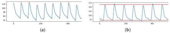
Figure 1.
Fraction of ABP signal (y-axis) over time (x-axis) with: (a) highlighted peaks (SBP, orange stars) and minimum points (DBP, green stars); (b) extracted SBP (mean of peaks) and DBP (mean of minimums).
Using Python’s ready-to-use function “scipy.signal.find_peaks”, peak detection was carried out. In order for the peaks to be detected, it is necessary to define a “prominence” (a sort of threshold for the height of the peaks). Prominence must be assessed on a case-by-case basis because the ABP range is flexible. This parameter was empirically chosen to be the difference between each ABP signal median and minimum value.
2.1. Database
The UCI dataset, also known as the Cuff-Less Blood Pressure Estimation Dataset, was used in this study due to its simplicity and readiness [11,12]. It was sourced from the MIMIC-II Waveform database, which tracks physiological measurements such as ABP and PPG [13]. The UCI dataset consists of 12,000 instances of simultaneous PPG, ABP, and ECG data from 942 patients, and was pre-processed by Kachuee et al. to smooth signals, eliminate unacceptable values, and autocorrelate PPG signals [11]. Pre-processing of the entire dataset was necessary before model training.
2.2. Preprocessing
Inspired by [3], the PPG recordings were filtered using a band-pass 4th order Butterworth filter with a bandwidth of 0.5 Hz to 8 Hz to exclude frequencies responsible for baseline wandering and high frequency noise. Moreover, in order to prevent motion artifacts and powerline artifacts, the ECG signal was filtered with an 8th order passband Chebyshev type 1 filter with a cut-off frequency of 2 Hz and 59 Hz. Then, the inputs were standardized instance-wise using a min-max normalization between 0 and 1.
It is crucial to emphasize that ABP was not altered in any manner in order to preserve pressure information. The SBP, DBP pressure readings and forecasts would have been inaccurate and information would have been lost if filters or pre-processing were applied.
2.3. Data Selection and Training Set Creation
Data are sampled at 125 Hz. Since the maximum duration of an instance is 10 min, each instance of ECG, PPG and ABP will have at most 75,000 data points. To have adequate information to forecast the overall trend and the impact of the ECG and PPG on ABP, all the instances were divided in segments of length of 8 s (1000 points), comparable to [5] (1024 points).
The signal segments extracted from the UCI dataset contain many highly distorted signals that prevented the deep learning model from properly mapping input signals to the corresponding ABP waveform and, thus, hinder correct SBP and DBP estimation. Experimentally, it was found that highly distorted signals typically lie on one of the following categories: SBP below 80 mmHg or over 190 mmHg; DBP below 50 mmHg and above 120 mmHg; blood pressure ranges () below 20 mmHg or above 120 mmHg. As a result, these ABP samples, together with their corresponding ECG and PPG signals, were removed from the dataset.
Afterwards, since the peaks of ECG, PPG, and ABP signals are frequently non-uniform, e.g., due to patient movements during acquisition, an additional data selection step has been performed, based on the standard deviation of peak heights and peak distances within each extracted signal. Here, some maximum values have been fixed to filter out noisy signals; Table 1 summarizes these thresholds for PPG, ECG, and ABP, respectively.

Table 1.
Pruning thresholds for the standard deviation of PPG, ECG, and ABP.
2.4. Input and Output of the Network
The PPG, ECG, VPPG = , and APPG = , each with a length of 1000 (8 s) time instants, has been fed, in this order, to a different network channel to make the input tensor with shape (1000, 4). On the other side, an ABP waveform lasting 8 s will be the network target, which the model must forecast. Figure 2 shows an example of input tensor (Figure 2a–d) and the relative ABP output to be predicted (Figure 2e).
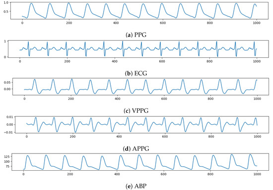
Figure 2.
Example of input vector over time (x-axis) composed, from top to bottom (y-axis), by: PPG, ECG, VPPG, APPG; and then the relative ABP to be predicted.
2.5. Extracted Signals Analysis
After the previously described preprocessing, thresholding and cleaning phases, 192,661 input tensors (each of 8 s) were obtained, for a total of 428.13 h of training data in total. It can be helpful to examine the SBP and DBP distribution of the extracted examples shown in Figure 3. Due to the thresholds defined during the extraction and selection of signal steps, it follows that the distributions are truncated where the upper and lower boundaries have been set. It can also be observed DBP is generally less dispersed than SBP (see Figure 3 right).
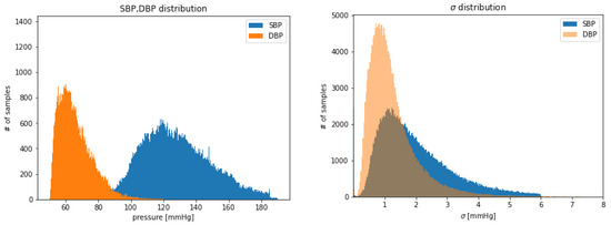
Figure 3.
Distribution of: SBP and DBP extracted values (left); of extracted values of SBP, DBP (right).
3. Network Architecture
Inspired by the great results of [3] and [5] our first idea was to use a “mixture” of the two models. However, since the architecture of [5] was huge (about 120 million of parameters), it is evident that this approach could not be the optimal one for the ABP prediction, especially looking at the network of [3] (just around 2 million parameters). Therefore, it was opted to use a series of Conv1D (with 128 filters and kernel size equal to 3), and BiLSTM layers.
Conv1D [14,15] are commonly used in time-series analysis because they can effectively extract temporal features from the data. This is particularly useful when dealing with noisy or variable data, where traditional statistical methods may not be effective.
Bidirectional Long Short-Term Memory (BiLSTM) [3] networks are also commonly used in time-series analysis because they can effectively capture both past and future information in the time-series.
The idea behind the model is to use a sort of “encoder–decoder” structure, based on the Conv1D layers, with the BiLSTM as a backbone, instead of a simple Multi Layer Perceptron as [5]. Also, a skip connection between and after the backbone to prevent the vanishing gradient was used. The resulting structure can be seen in detail in Figure 4.
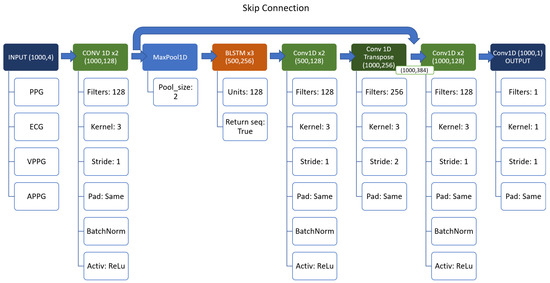
Figure 4.
Structure of the first network.
4. Experiments and Results
All of the examples were randomly shuffled before the network training began (using the same seed for each experiment, for sake of comparability), and the training set was made up of 80% of the data, while validation and testing subsets received 10% each, respectively.
All the experiments were performed using Adam optimizer Keras default configuration [16,17] and 30 epochs. Due to the presence of the MaxPool layer, the stride of the Conv1DTranspose layer must be set to 2 to match the input/output dimensions, and keep the same number of parameters in the network.
To stick with the state of the art, two metrics—Mean Absolute Error (MAE) as the observed metric and Mean Square Error (MSE) as the loss function for the model—were used in all the experiments. Overall, while other loss functions may be used for time-series regression, MSE is an effective choice due to its simplicity, interpretability, and effectiveness in capturing the error between predicted and actual values over time.
The first experiment was made using the architecture of Figure 4, which employed 64 input batches, a Max Pool layer, and 3 BiLSTM layers. Results in terms of MAE and MSE, for both training and validation, are shown in Figure 5.
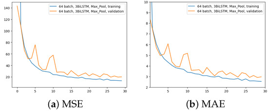
Figure 5.
Error (y-axis) over epochs (x-axis) for the first experiment (batch size = 64, 3 BiLSTM and MaxPool layer): (a) MSE on training (blue line) and validation (red line) sets; (b) MAE on training (blue line) and validation (red line) sets.
The second experiment aimed to comprehend the importance of removing the MaxPool layer. Here, 3 BiLSTM and 64 input batches were still used. The time for the computation increased from 2.5 h to 4 h. The outcomes are displayed in Figure 6.
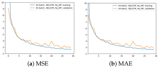
Figure 6.
Error (y-axis) over epochs (x-axis) for the second experiment (batch size = 64, 3 BiLSTM and no MaxPool layer): (a) MSE on training (blue line) and validation (red line) sets; (b) MAE on training (blue line) and validation (red line) sets.
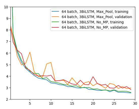
Figure 7 shows a comparison among these two network configurations with regard to the MAE metric. It can be seen that removing the layer has almost no impact on the regression performance. With a slightly more pronounced difference at early epochs, the two configurations appear to converge in the same way at the latest epochs. Since removing the MaxPool layer does not seem to bring any noticeable improvements, in all future experiments this layer will be used due to its much faster network training time.
In the third experiment, just two BiLSTM were implemented to assess the impact of different number of BiLSTM layers; the rest remains as per the first experiment (i.e., 64 input batches and Max Pool layer). Figure 8 displays the outcome in comparison to the other two experiments for the two metrics. It is evident that using only two BiLSTM reduces performance across the board. The validation MAE never achieves the outcomes of the first two experiments.
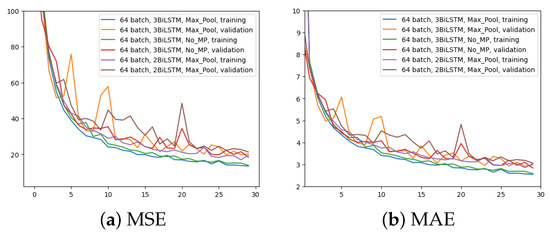
Figure 8.
Error (y-axis) over epochs (x-axis) for the third experiment (batch size = 64, 2 BiLSTM and MaxPool layer) compared to the previous two networks: (a) MSE on training and validation sets; (b) MAE on training and validation sets.
The last experiment aimed to highlight the effects of increasing the batch size to 256 with MaxPool and 3 BiLSTM layers. Figure 9 yields the results. Even though the network is still learning, it does not appear to converge as quickly as it did in the previous experiments, as it is evident just by looking at Figure 9a. However, at higher epochs, the MAE training trend appears to converge to similar values. The validation MAE, however, never falls below the other model with a 64 batch size, as can be seen by looking at Figure 9b.
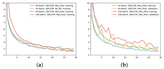
Figure 9.
Comparison of MAE (y-axis) over epochs (x-axis): (a) All networks, only training; (b) first and last network configurations, training and validation.
In conclusion, the ablation study that performed pruning on some parts of the initial network proved that the architecture shown in Figure 4 is the best performing one. Indeed, it reaches lower MAE values than the third and fourth configurations and requires a quite shorter training time than the second network, as previously stated. For sake of completeness, after choosing the ideal structure and parameters, it is possible to see some examples of the model predictions using random inputs from the test set, in Figure 10.
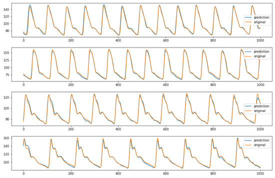
Figure 10.
Examples of predicted ABP (y-axis) over time (x-axis) from the first network configuration (64 batch size, MaxPool and 3 BiLSTM layers). The predictions are relative to random inputs from the test set, to show the network capability of reproducing different kind of waveform.
5. Conclusions
This paper aimed to build a lightweight neural network model to predict 8 s of ABP signal, using the “Cuff-Less Blood Pressure Estimation Dataset”. At this purpose, a novel network, based on Conv1D as encoder/decoder block and BiLSTM as backbone, was proposed. The initial architecture was designed using 64 input batch size, MaxPool and 3 BiLSTM layer. Then, three additional network configurations were presented by means of an ablation strategy, and their performances were compared in terms of MAE and MSE metrics. The best performing model was the initial one, which achieved, on test data, a MAE of around 2.97 mmHg.
The main contribution of this paper is to have given a simple way of predicting ABP and lay the foundations for a transfer of research results on possible portable/wearable medical devices. One of the next steps will be to apply this method to real-world scenarios, where data are often more irregular and noisy. Furthermore, it may be interesting to use this method to derive SBP and DBP directly without predicting the entire ABP waveform. Also, the use of a larger database, such as the new MIMIC IV, could also improve performance and generalization.
Author Contributions
Conceptualization, V.R. and E.P.; methodology, F.D., G.C. and V.R.; software, F.D.; validation, F.D., V.R. and G.C.; formal analysis, F.D. and G.C.; investigation, F.D.; resources, E.P. and V.R.; data curation, F.D.; writing—original draft preparation, F.D. and V.R.; writing—review and editing, V.R.; visualization, F.D.; supervision, V.R., E.P. and G.C.; project administration, E.P and V.R.; funding acquisition, E.P. and V.R. All authors have read and agreed to the published version of the manuscript.
Funding
This research has been partly funded by the BrS-AI-ECG project of the Italian Ministry of Foreign Affairs and International Cooperation. Dr. Randazzo also acknowledges funding from the research contract no. 32-G-13427-2 (DM 1062/2021) funded within the Programma Operativo Nazionale (PON) Ricerca e Innovazione of the Italian Ministry of University and Research.
Institutional Review Board Statement
Not applicable.
Informed Consent Statement
Not applicable.
Data Availability Statement
The data presented in this study are openly available in The UCI dataset, also known as the Cuff-Less Blood Pressure Estimation Dataset [11,12].
Acknowledgments
Delrio acknowledges Eurecom for support in his PhD research.
Conflicts of Interest
The authors declare no conflict of interest.
References
- Parati, G.; Stergiou, G.S.; Dolan, E.; Bilo, G. Blood pressure variability: Clinical relevance and application. J. Clin. Hypertens. 2018, 20, 1133–1137. [Google Scholar] [CrossRef] [PubMed]
- Ilies, C.; Bauer, M.; Berg, P.; Rosenberg, J.; Hedderich, J.; Bein, B.; Hinz, J.; Hanss, R. Investigation of the agreement of a continuous non-invasive arterial pressure device in comparison with invasive radial artery measurement. Br. J. Anaesth. 2012, 108, 202–210. [Google Scholar] [CrossRef] [PubMed]
- Paviglianiti, A.; Randazzo, V.; Villata, S.; Cirrincione, G.; Pasero, E. A Comparison of Deep Learning Techniques for Arterial Blood Pressure Prediction. Cogn. Comput. 2021, 14, 1689–1710. [Google Scholar] [CrossRef] [PubMed]
- Ibtehaz, N.; Mahmud, S.; Chowdhury, M.E.H.; Khandakar, A.; Salman Khan, M.; Ayari, M.A.; Tahir, A.M.; Rahman, M.S. PPG2ABP: Translating Photoplethysmogram (PPG) Signals to Arterial Blood Pressure (ABP) Waveforms. Bioengineering 2022, 9, 692. [Google Scholar] [CrossRef] [PubMed]
- Mahmud, S.; Ibtehaz, N.; Khandakar, A.; Tahir, A.M.; Rahman, T.; Islam, K.R.; Hossain, M.S.; Rahman, M.S.; Musharavati, F.; Ayari, M.A.; et al. A Shallow U-Net Architecture for Reliably Predicting Blood Pressure (BP) from Photoplethysmogram (PPG) and Electrocardiogram (ECG) Signals. Sensors 2022, 22, 919. [Google Scholar] [CrossRef] [PubMed]
- Randazzo, V.; Ferretti, J.; Pasero, E. Anytime ECG Monitoring through the Use of a Low-Cost, User-Friendly, Wearable Device. Sensors 2021, 21, 6036. [Google Scholar] [CrossRef] [PubMed]
- Cirrincione, G.; Randazzo, V.; Pasero, E. A neural based comparative analysis for feature extraction from ECG signals. In Neural Approaches to Dynamics of Signal Exchanges; Springer: Singapore, 2020; pp. 247–256. [Google Scholar]
- Athaya, T.; Choi, S. An Estimation Method of Continuous Non-Invasive Arterial Blood Pressure Waveform Using Photoplethysmography: A U-Net Architecture-Based Approach. Sensors 2021, 21, 1867. [Google Scholar] [CrossRef] [PubMed]
- Cheng, J.; Xu, Y.; Song, R.; Liu, Y.; Li, C.; Chen, X. Prediction of arterial blood pressure waveforms from photoplethysmogram signals via fully convolutional neural networks. Comput. Biol. Med. 2021, 138, 104877. [Google Scholar] [CrossRef] [PubMed]
- Paviglianiti, A.; Randazzo, V.; Cirrincione, G.; Pasero, E. Neural recurrent approches to noninvasive blood pressure estimation. In Proceedings of the 2020 International Joint Conference on Neural Networks (IJCNN), Glasgow, UK, 19–24 July 2020; IEEE: Piscataway, NJ, USA, 2020; pp. 1–7. [Google Scholar]
- Kachuee, M.; Kiani, M.M.; Mohammadzade, H.; Shabany, M. Cuffless Blood Pressure Estimation Algorithms for Continuous Health-Care Monitoring. IEEE Trans. Biomed. Eng. 2017, 64, 859–869. [Google Scholar] [CrossRef] [PubMed]
- Kachuee, M.; Kiani, M.; Mohammadzade, H.; Shabany, M. Cuff-Less Blood Pressure Estimation. UCI Machine Learning Repository. 2015. Available online: https://archive.ics.uci.edu/dataset/340/cuff+less+blood+pressure+estimation (accessed on 30 June 2023).
- Goldberger, A.L.; Amaral, L.A.N.; Glass, L.; Hausdorff, J.M.; Ivanov, P.C.; Mark, R.G.; Mietus, J.E.; Moody, G.B.; Peng, C.K.; Stanley, H.E. PhysioBank, PhysioToolkit, and PhysioNet: Components of a New Research Resource for Complex Physiologic Signals. Circulation 2000, 101, e215–e220. [Google Scholar] [CrossRef] [PubMed]
- Ferretti, J.; Barbiero, P.; Randazzo, V.; Cirrincione, G.; Pasero, E. Towards uncovering feature extraction from temporal signals in deep CNN: The ECG case study. In Proceedings of the 2020 International Joint Conference on Neural Networks (IJCNN), Glasgow, UK, 19–24 July 2020; IEEE: Piscataway, NJ, USA, 2020; pp. 1–7. [Google Scholar]
- Ferretti, J.; Randazzo, V.; Cirrincione, G.; Pasero, E. 1-D convolutional neural network for ECG arrhythmia classification. In Progresses in Artificial Intelligence and Neural Systems; Springer: Singapore, 2021; pp. 269–279. [Google Scholar]
- Abadi, M.; Agarwal, A.; Barham, P.; Brevdo, E.; Chen, Z.; Citro, C.; Corrado, G.S.; Davis, A.; Dean, J.; Devin, M.; et al. TensorFlow: Large-Scale Machine Learning on Heterogeneous Systems. arXiv 2016, arXiv:1603.04467. [Google Scholar] [CrossRef]
- tf.keras.optimizers.Adam | TensorFlow v2.11.0. Available online: https://www.tensorflow.org/ (accessed on 30 June 2023).


Disclaimer/Publisher’s Note: The statements, opinions and data contained in all publications are solely those of the individual author(s) and contributor(s) and not of MDPI and/or the editor(s). MDPI and/or the editor(s) disclaim responsibility for any injury to people or property resulting from any ideas, methods, instructions or products referred to in the content. |
© 2023 by the authors. Licensee MDPI, Basel, Switzerland. This article is an open access article distributed under the terms and conditions of the Creative Commons Attribution (CC BY) license (https://creativecommons.org/licenses/by/4.0/).