Abstract
Biogas is an important driver in carbon-neutral energy sources. Many biogas digester setups, however, are not well optimized and waste energy or fail to maximize their gas output potential. To optimize these systems, a framework was developed to measure and predict digester systems’ efficiencies by closely monitoring fluid movements. This framework includes a numerical calculation of fluid behavior (Computational Fluid Dynamics (CFD)), and Deep Learning to estimate the fluid shear-rates introduced by the agitator’s action. Additionally, a novel measurement system is presented that can measure the same metrics, as simulated, in real-world environments. Lastly, an outlook is given that presents the options and extensions of the presented setup to reduce prediction error, minimize measuring efforts further, and recommend optimization approaches to the operator.
1. Introduction
Carbon-neutral energy sources play a crucial role in mitigating climate change. Statistics show that the energy generated from biomass in Germany has been continuously rising since 1991 [1]. These systems, however, are often built up and operated without an exact setup or analysis of the maximum efficiency. Thus, these system often do not reach their full potential [2]. To produce energy, these systems agitate a fluid that consists of animal waste, energy crops, organic waste, and other materials, in varying amounts [3]. The agitation action keeps the fluid fermenting, thus producing a valuable biogas that consists mainly of methane () and carbon dioxide (), and small amounts of other gases. Biogas is used in many different applications, such as heating or locomotion [4]. Effective agitation is essential during the fermentation process [5]. On the one hand, over-agitation wastes energy; on the other hand, under-agitation risks the formation of solid or foamy swimming layers that can result in the fermentation process stopping completely. In addition to the high variance in biogas fluid characteristics, these systems are set up with many varying factors, such as the type of rotor used, the size of the rotor, the height and diameter of the agitation vessel, and if the vessel is equipped with features to aid agitation by increasing turbulence. Having one setup for every biogas digester is impossible, individual analyses will probably increase the efficiency of these systems. This work approaches the optimization of process by deploying deep learning. The amount of data required to properly train a neural network far outscales what is collectible in a reasonable timeline. For this, many different systems will have to be located and measured for extended periods. This problem can be overcome by computationally generating the required data. Computational Fluid Dynamics is a common practice to understand the flow of fluids in any configuration. This approach can be used to generate knowledge about the flow behavior in biogas power plants. A sim-to-real transfer is achieved by tweaking the pre-trained Artificial Neural Network (ANN) with real-world measurements.
This work presents the methodology used to design, simulate, measure, and predict agitation efficiencies using deep learning. First, the methodology of this approach is presented. The Computer-Aided Design and Computational Fluid Dynamics setup are outlined to simulate systems and generate data for the deep learning phase. Next, post-processing steps are implemented to convert simulation results to data that can also be obtained with a real-world measuring system. Then, the Neural Network Architecture is presented, where three commonly used approaches are implemented and compared. The Section 2 is concluded with a detailed look at the three Neural Network Architectures and their performances in the presented problem. After the Section 2, a Wireless Sensor Network (WSN) to measure real-world systems is outlined. Its purpose is to measure real-world systems, and to refine the neural network predictions. In the outlook, future work is described that will further improve the presented system by minimizing measurement effort and helping the operator to create an optimal agitation setup.
2. Methodology
In this section, the methodology used to set up simulation environments, numerical simulation, post-processing, the Neural Network Architectures, and deep learning is explained. The first part outlines the development of the 3D models that are to be used in the numerical analysis. Next, the numerical analysis in OpenFOAM is explained, including the setup of fluid properties, mesh-movements, mesh-boundary conditions, and information about the overall analysis process. The subsequent section outlines further processing of the results of numerical analysis using ParaView. These operations are crucial to align the data formats of real-world measurements and simulation. After the CFD post-processing, three artificial-neural-network architectures are outlined. Lastly, the performance of these networks on training and test data is presented.
2.1. CAD
This section outlines the Computer-Aided Design (CAD) of the biogas plant models used for this work. Two different models were implemented, from which three different simulation cases were derived.
Figure 1 shows the different models and their stirrer setups. A 3D model of the Landia-POP-I Slurry Mixer was implemented in a top model. The same mixer model was modified to allow for more degrees of freedom in regard to the rotors’ position. For this, the body of the rotor was removed and all open faces were patched. This resulted in an abstract floating stirrer that can be placed anywhere in the vessel, without a disruption of the flow caused by the mixers body. Surrounding the stirrer are the vessel walls, and top and bottom lids. Depending on the type of biogas plant, these can be rounded (Figure 1 top) or fitted with plates (Figure 1 bottom). Not shown in the figure above are the top lid, which acts as the vessel walls, and the bottom lid, which keeps fluid from spilling out.

Figure 1.
Renders of two different plant model setups. The top lids were removed for this visualization. (Top) shows a standard fermenter with a 28 m vessel diameter and filling height of 7 m (left) and a Landia POP inclined blade stirrer [6] that launches the fluid perpendicular from the vessel wall (right). (Bottom) shows an agitation setup that is based on a real-world system where fluid-tracking measurements were taken in the past [7]. The vessel diameter is 11 m, vessel fill height is 2 m (left), and a reduced Landia POP inclined blade stirrer is used to launch the fluid in a parallel motion to the vessel walls.
2.2. Computational Fluid Dynamics
For this work, three simulation cases were developed, where one is based on a previously measured system [7]. One challenge when simulating biogas plants is the non-Newtonian fluid’s behavior. The shear-thinning fluid decreases its viscosity when a force is applied to it, varying its behavior in comparison to most fluids, like water. Additionally, these fluids exact properties that vary from their compositions and other variables, e.g., animal feed. To approximate the fluid’s shear-thinning viscosity behavior, the approach of Fosca Conti et al. [8] was followed. Thus, for this simulation, the power-law model for the viscosity of Oswald–deWaele was chosen [9].
with the kinematic viscosity and a consistency factor , which equals a kinematic consistency factor. (The kinematic consistency factor k is the quotient of the consistency factor K and the fluid’s density ; ). of m2s−1, a power-law index of , where , describes the fluid as shear-thinning. The fluid’s kinematic viscosity limits are set to m2s−1 and m2s−1.
This simulation aims to compute field velocities v, and, with a custom post-processing-module, field shear-rates . After the definition of fluid behaviors, the CAD models of all parts involved in fluid movements are implemented in a simulation case.
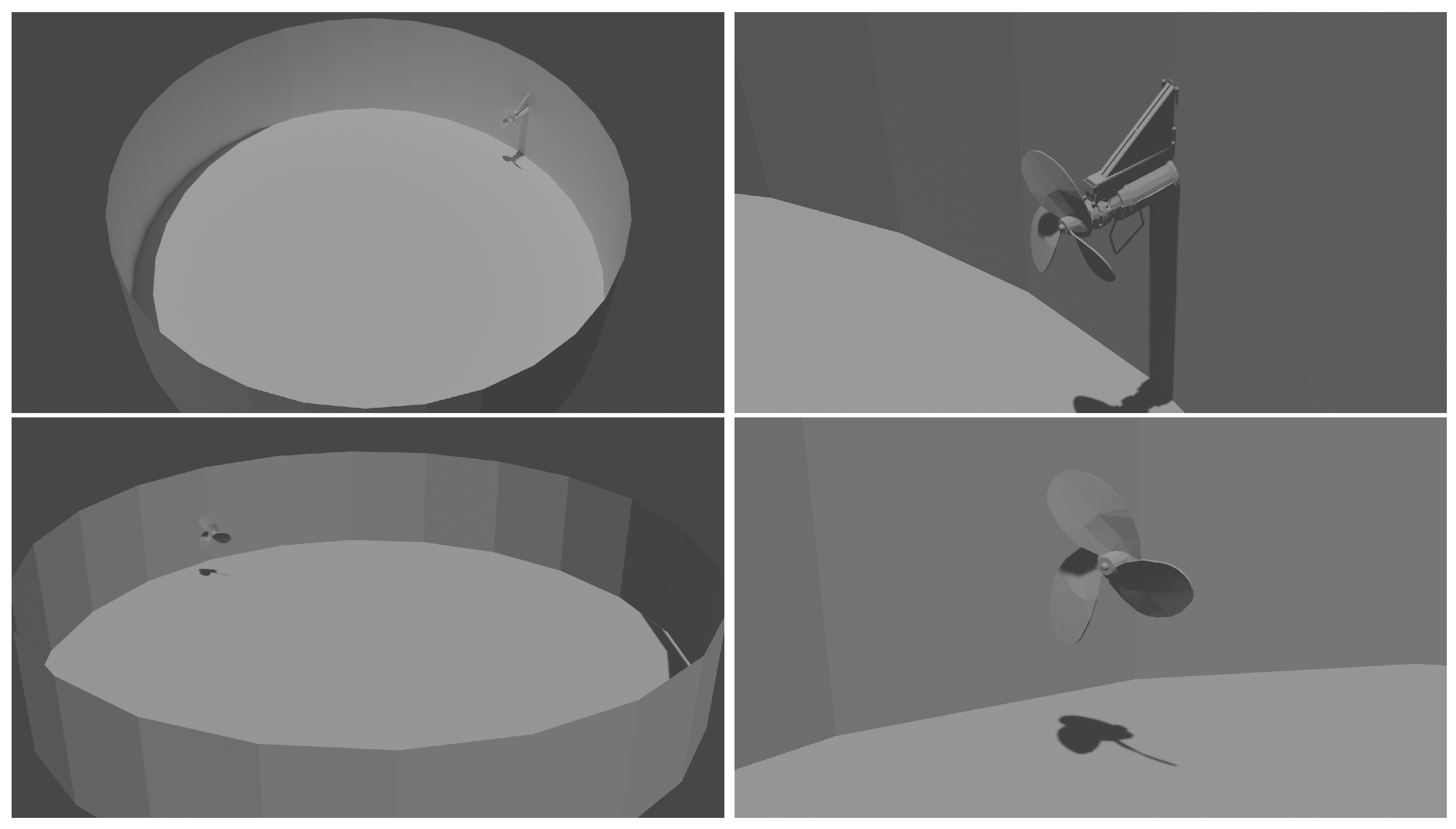
Figure 2 shows a CFD setup used for one of three case setups that have been created for this work. Additionally, the meshing of all the parts’ features is highlighted.
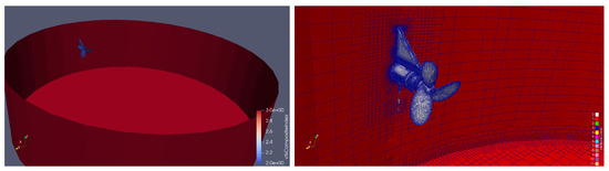
Figure 2.
ParaView capture of a simulation case. Left shows a case setup of a previously simulated agitation system. The displayed vessel’s radius is m and its height is m. right side shows a magnification view of the setup’s agitator, with a m rotor radius and rated rotational speed configured to 150 RPM.
For two cases, the Landia POP-I Slurry Mixer [6] was designed as per manufacturer’s specifications, to describe rotating speeds of 150, and 300 , depending on the chosen gearing. In a third case, a faulty agitator setup is implemented. Here, the rotor spins in the wrong direction with a very low rotating speed of 75 . For all three cases, Arbitrary Mesh Interfaces (AMI) were implemented to cause rotor blades to spin and inflict movement on the fluid. Other case properties include:
- Turbulence model: Only the overall resulting fluid flow is of interest. The turbulence behavior is set to laminar.
- Transient/steady state: The start-up behavior of the system is of interest; a transient solver has been chosen.
- Fluid compressibility: With the overall slow fluid velocities, we can safely assume an incompressible fluid.
With the presented case characteristics, OpenFOAM’s pimpleFoam-solver was chosen [10]. The CFD Simulation was carried on a Workstation PC, equipped with an Intel Core i5-8600k hexa-core processor [11]. Each case took five days of continuous computation to complete 100 of simulation time. Data points of were captured in at least one-second time intervals.
2.3. CFD Post-Processing
After computing the required metrics, namely velocity v and shear rate , virtual mass- and volume-less nodes are generated within the fluid using ParaView’s Particle Tracer filter. These nodes follow the local velocity fields of the fluid and closely replicate the behavior of a real-world flow follower. The real-world measurement technique is outlined in Section 3.
Figure 3 shows the startup of an agitation system and the effects on the mass-less particles (blue nodes) floating in the fluid (hidden). The presented setup was developed in ParaView v5.10 [12], utilizing the engine’s Python scripting interface. Numerous equidistant lines are created inside the vessel, which are used as seed sources for the particle tracer. Nodes created like this can then be used for further processing in Deep-Learning Applications.
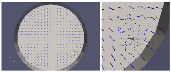
Figure 3.
ParaView setup for CFD post-processing with particle tracer nodes at simulation 1.5 s after system start-up. Left shows a top-down view of an agitation setup, with m vessel radius and 2 m height. The fluid is hidden. Mass-less are shown in blue. Right figure shows a magnified view of the rotor ( m radius, 150 RPM), which is pointed north in this case. These figures show the system in startup, where particles around the rotor have already been affected by its agitation motion.
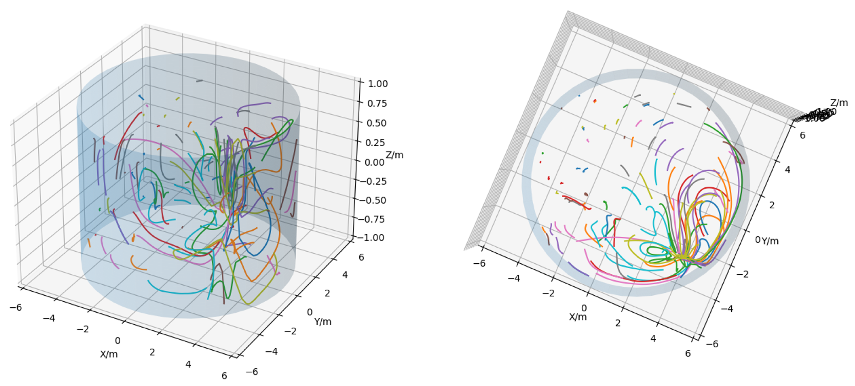
Figure 4 shows two perspectives of a trajectory plot with 100 random particles. Since all lines in this figure span the same time interval, longer lines denote particles with a greater average velocity. With this information, the rotor’s location can be gauged. To decouple absolute node positions and related velocities, as seen in Figure 4, incremental position information is derived from absolute positions. This step effectively transforms the position data into local particle velocities u.
where represents the particles position in a three-dimensional space, and is the time interval between two position measurements. For this work, s.
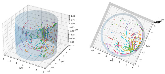
Figure 4.
3D Plot of 100 randomly chosen particle trajectories from the system seen in Figure 3. The cylinder approximates vessel walls and the colored lines denote the particles trajectory over the whole 100 s simulation time. Right shows the same 3D plot viewed from a top-down angle.
2.4. Neural Network Architecture
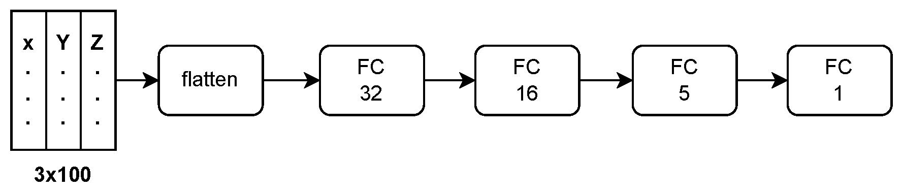
In this work, widely used regression network architectures are compared to estimate fluid shear-rates . Fully Connected Neural Networks (FCNN) are simple setups, where the raw input (described in previous Section 2.3) is flattened and fed into the first dense layer of the FCNN. Subsequently, three hidden layers follow, with thirty-two, sixteen, and five neurons, before the network terminates with a single neuron that reflects its prediction of the mean trajectory shear-rate .
The Fully Connected Neural Network architecture is shown in Figure 5.

Figure 5.
Fully Connected Neural Network (FCNN) architecture, with three densely connected hidden layers of thirty-two, sixteen, and five neurons. The activation function of the hidden layers is the Rectified Linear Unit (ReLU). The output layer consists of one single neuron with linear activation.
Another widely used network architecture is the Convolutional Neural Network (CNN), which adds various convolution- and max-pooling layers, preceding densely connected layers, to enhance features. Two different architectures for this type of network were developed.
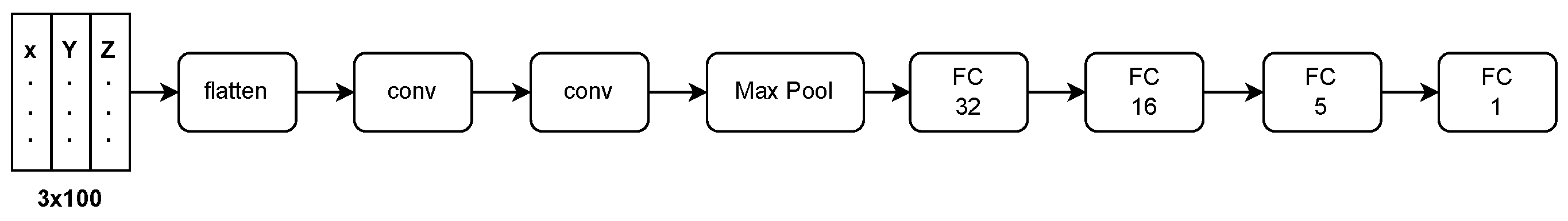
The first CNN will be referred to as 1D-CNN, because, like the FCNN, it starts with a flattening layer, resulting in Rank-1 tensor operations. Next, two 1D convolution layers, with kernel sizes of ten and seven, follow. After convolution, global max-pooling is applied, after which the network proceeds with the same three dense layers as presented for the FCNN (32, 16, 5, and 1 neurons).
Figure 6 shows the architecture of the 1D Convolutional Neural Network.

Figure 6.
Convolutional Neural Network (CNN) with flattening operation in the first layer, referred to as 1D-CNN in this work. The flattening follows the Rank-1 Tensor operations convolution with a size of 10 kernels, convolution with a size of 7 kernels, global max-pooling and the same densely connected layers as described in Figure 5. All hidden layers are configured with Rectified Linear Unit (ReLU) activation; the single neuron output layer has linear activation.
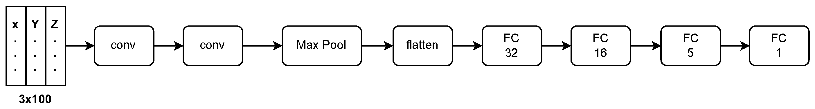
In contrast, a Rank-2 Tensor based CNN was implemented. This architecture follows the same outline as 1D-CNN, using 3 × 3 convolution kernels. The main difference is that flattening is applied right before the first dense layer.
The 2D-CNN architecture is shown in Figure 7.

Figure 7.
Convolutional Neural Network (CNN) with flattening operation in the last layer before the dense layers, referred to as 2D-CNN in this work. Input data are fed into two Rank-2 Tensor convolution layers with 3 × 3 kernels, followed by a global max-pooling layer, before feeding these into the same densely connected layers as described in Figure 5. All hidden layers are configured with Rectified Linear Unit (ReLU) activation; the single neuron output layer undergoes linear activation.
2.5. Deep Learning
All networks outlined in the last section (Section 2.4) were trained over 150 epochs. The Mean-Squared Error (MSE) loss function was chosen for these regression architectures. With the framework explained in Section 2.1, Section 2.2 and Section 2.3, datasets of complete length (100 s simulated time span, and 1 Hz update rate) were generated. Datasets were split into 80% training data, and 20% test data, which are only used for validation tests.
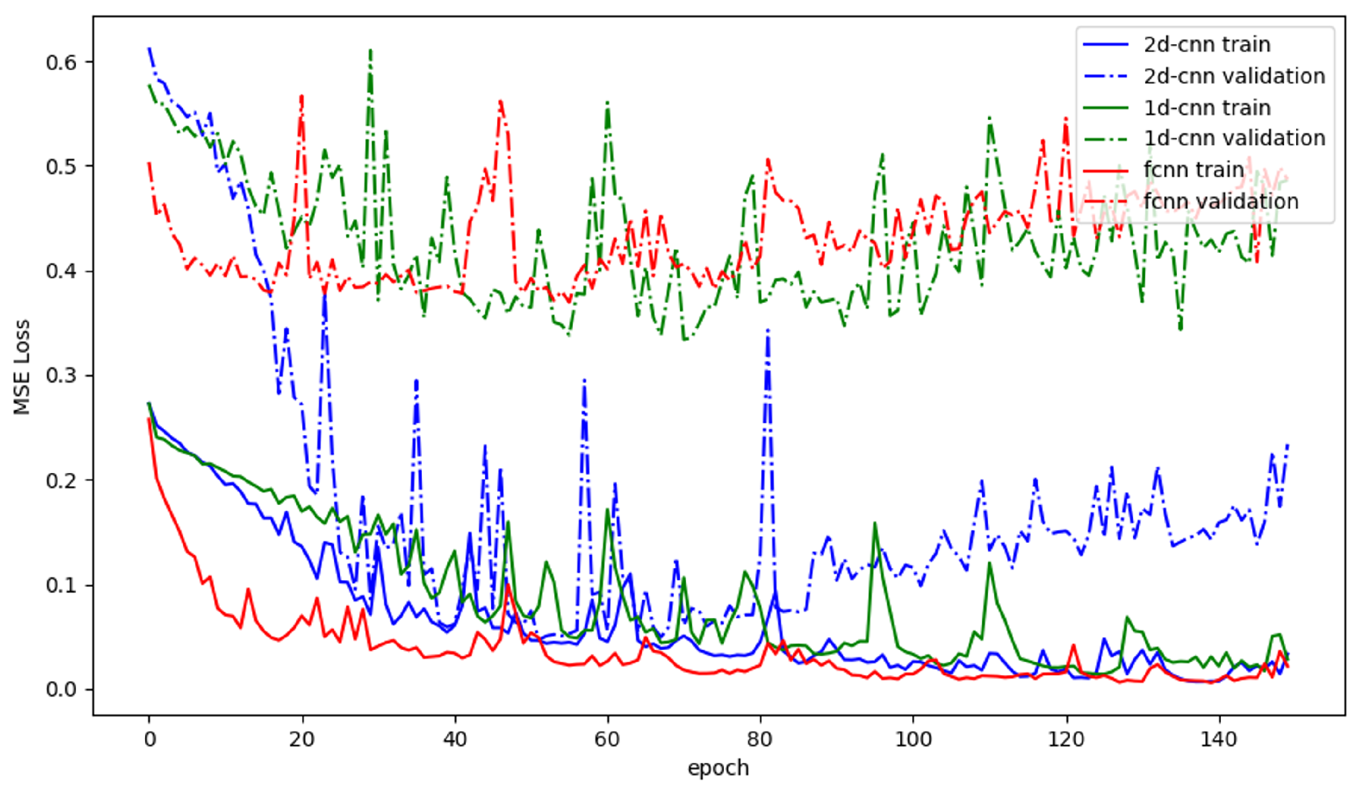
Figure 8 show all three network performances throughout the 150 epochs of training. The FCNN shows no meaningful improvements after around 20 training epochs, where the loss stays around MSE. Additionally, the FCNN shows signs of overtraining after around 60 training epochs: the loss in the validation set increased, where as the loss in the training set continued to decrease. The 1D-CNN performed very similarly to the FCNN, although it needs around 40 training epochs to achieve the same performance of around MSE. After around 100 training epochs, this network shows sings of overtraining, with the MSE not deviating much from the FCNN’s. The FCNN and the 1D-CNN never reached validation losses close to the ones reached on the training-sets; the difference in the validation set is always bigger than MSE. Lastly, the 2D-CNN performs the best for the presented problem. After around 50 training epochs, the network reaches its best performance with the validation loss function decreasing to around MSE, where the loss functions on the training and validation sets align. Like the other two, this network starts showing sings of overtraining after around 70 training epochs. All three networks, especially the 2D-CNN, show very high variability in their losses throughout the training. This could originate from a lack of training data.
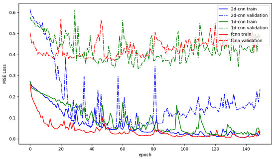
Figure 8.
Mean-Squared-Error losses of the presented deep learning architectures. Solid lines denote the losses on the training set of the network, whereas the dashed lines denote the losses on a test set. Red lines show losses of the FCNN; green lines refer to the 1D-CNN; lastly, blue lines show the losses of the 2D-CNN.
Since the single difference between the 1D- and 2D-CNN is the position of the flattening layers, this compirison shows how valuable the convolution and pooling operations on the 3D space data in the presented problem are.
3. Real-World Measurements
After focusing on the computational methods for data collection, this chapter focuses on real-world measurements and post-processing to refine the same deep-learning models as explained in Section 2.4.
3.1. Real-World Measuring Setup
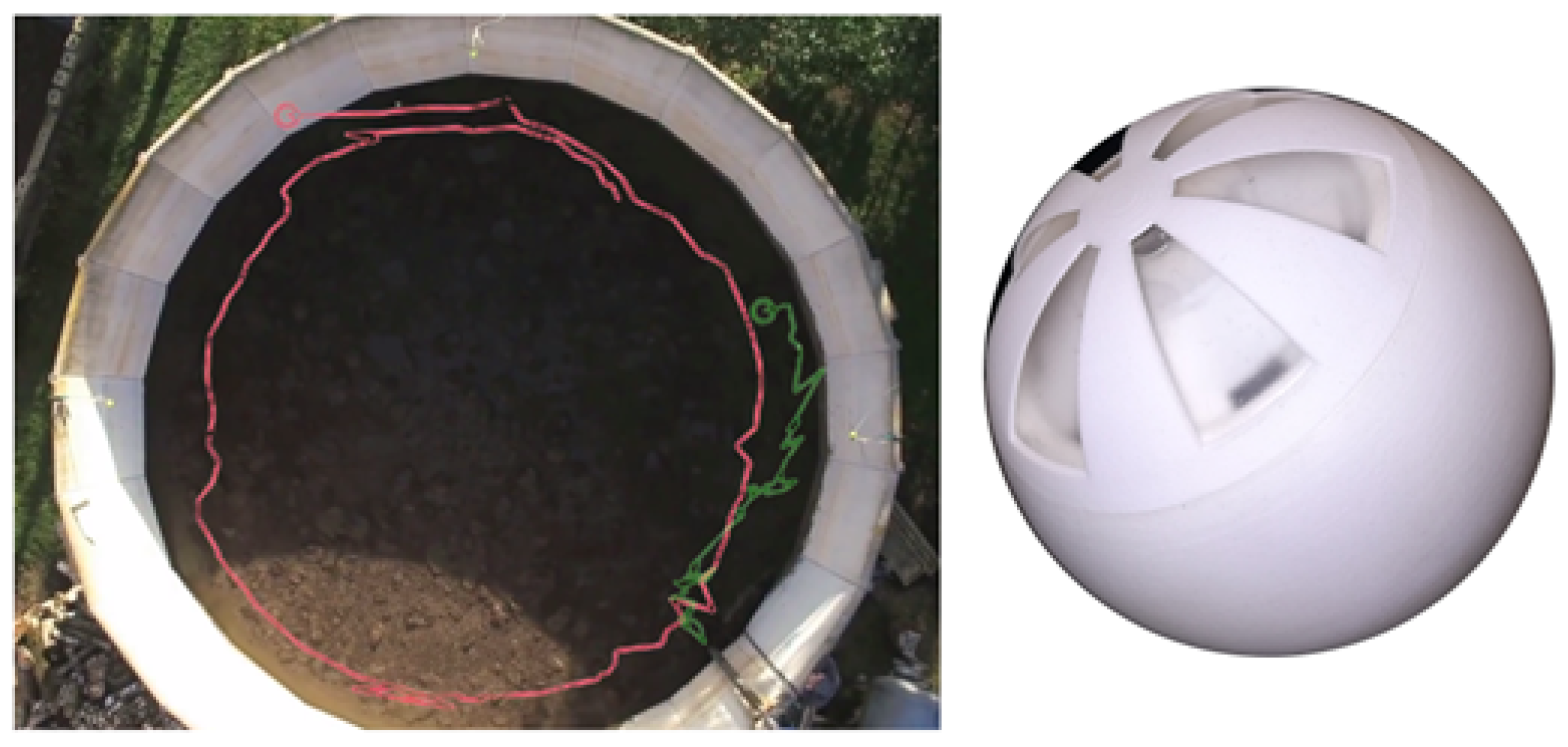
Figure 9 left shows a system evaluation made in the past [7]. This system was able to follow the behavior of the fluid on its surface, although it offered no insight into sub-surface flow characteristics. To achieve this, the measurement system was extended in the NeoBio research project [13]. This updated node is shown in Figure 9 right. It introduces important features to extend the existing functionality. This version can vary its volume to mass proportions by moving a flexible membrane, enabling it to sink, come up to the fluid surface, and, in a neutral setting, follow the surrounding fluid’s motion. Additionally, the fluid’s conductivity is measured, which may provide further insights into fluid compositions and help specify fluid properties for computational analysis and simulation.
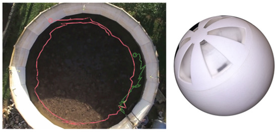
Figure 9.
Left shows an overlay of a past measurement with a revision 1 of the measurement system on a top-down photo of the measurement in progress. Anchor nodes are shown on the vessel’s west-, north- and east-facing rims. Right shows an updated version of the sensor particle that can measure fluid behavior below the fluid’s surface.
For the complete measuring setup, the node seen in Figure 9 right, is accompanied by anchor nodes mounted on the vessel side walls and a central data collection system, called backbone. The anchor nodes are shown in Figure 9 left.
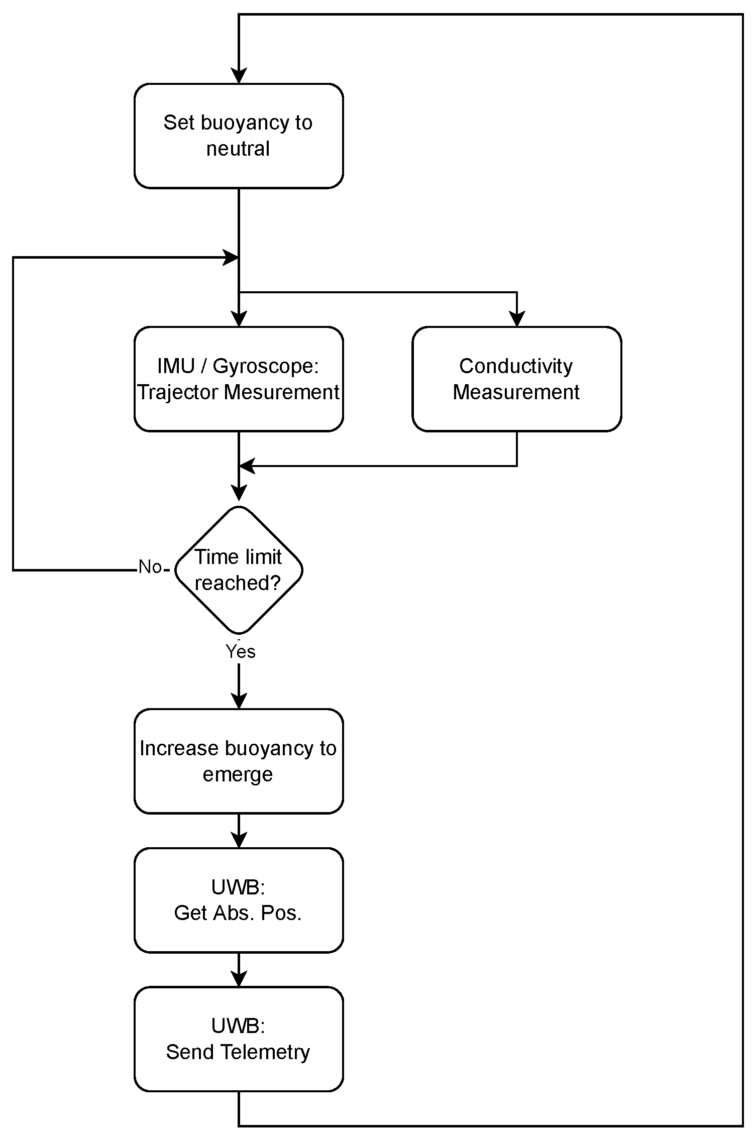
Figure 10 outlines the real-world data collection methodology.The sensor follows the fluid movements by setting the sensors’ buoyancy to neutral, so it follows the surrounding fluid’s flow. While the sensor is submerged, the movement is tracked using an inertial measurement unit (IMU) that integrates accelerations into an absolute trajectory [14]. Since this method of movement tracking is only accurate for a short time, the sensor node will frequently increase its buoyancy, letting itself rise to the substrate surface. From there, the WSN locates its absolute position in the fermenter using ultra-wideband (UWB) localization [15]. Next, all gathered data from previous dive are sent to the backbone, again using the UWB interface. After all data are off-loaded to the backbone, the sensor node will return to measuring mode, restarting the cycle.

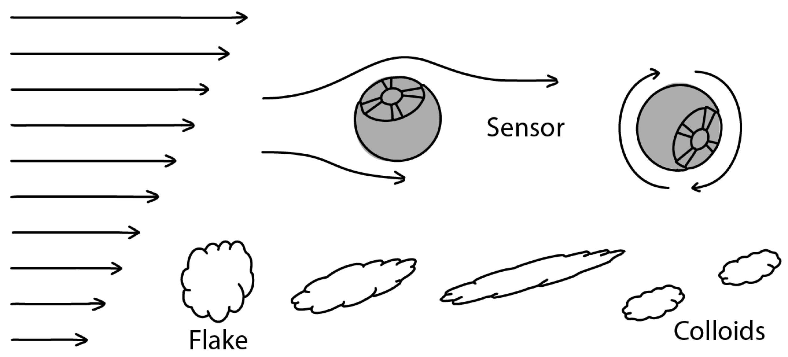
Figure 10.
Shear-rate measurement concept utilizing the sensors’ inertial measurement unit and gyroscope, and the same shear-rate effect on biogas substrate flakes, which are forced to break up into colloids [13].
3.2. Real-World Measurement Post-Processing
To use gathered datasets for deep-learning (see Section 2.4), they have to be converted into the same format, as explained in Section 2.2. Most importantly, this includes calculating shear-rates along the sensor’s trajectory. In Section 2.2, the simulated measuring nodes were defined with no volume and mass, and thus did not have inertia. Since this cannot be achieved in the real world, it has to be taken into account.
Figure 11 top outlines the effect of fluid shear-rates on a real-world sensor flowing with a liquid stream. Arrows on the left denote liquid flow velocities, which are increasing from bottom to top. The difference in the fluid speeds on the sensor’s surface will cause it to spin. This spin can be detected by the sensor’s IMU, and gyroscope. Figure 10 bottom shows the effect of the same change in fluid velocities on flakes that is found in a biogas substrate. These flakes are not rigid, like the sensor, and thus are elongated by the different forces applied to it until one flake breaks up into smaller colloids.

Figure 11.
Real-World Measurement methodology to track fluid movement and substrate conductivity.
4. Conclusions and Outlook
This work presented a framework for setting up, extracting and pre-processing data from simulated as well as real-world biogas plants. In addition, three deep-learning models were presented that, based on the generated data, predict a biogas plant’s agitation efficiency via its shear-rate. The presented 2D-CNN is capable of predicting shear rates with a Mean-Squared Error (MSE) of less than MSE, although all three models show signs of overtraining after 80 epochs. To gauge the accuracy of these systems in the real world, a framework for measuring these metrics in real-world environments was developed, although this could not be tested due to semiconductor shortages and the COVID-19 pandemic. Since the full range of biogas characteristics heavily depend on numerous factors, it is hard to specify these in a mathematical model for a Computational Fluid Dynamics (CFD) simulation. More research and a standardized model for a wide range of biogas plant setups will help to achieve results that can mimic real-world systems more closely.
Physics-Informed Neural Networks (PINNs) are a novel type of Deep-Learning setup that is specifically designed to predict physics problems and may increase the performance of the models presented here. In addition to PINNs, other features will be implemented using other deep-learning techniques. To further reduce the number of measurements required for each system, and increase the energy-efficiency of the real-world measuring system, Time Series Forecasting will be utilized to predict node trajectories.
Another problem to solve is the actual optimization of a real-world setup. Since the framework presented here only shows how well a system is performing, the optimization process is left to the user. A Recommender System will be implemented to solve this problem. This system will provide approaches to optimize agitation by, for example, suggesting optimal agitator settings or positions.
Author Contributions
Conceptualization, A.H., P.G., S.A., L.B. and S.R.; methodology, A.H.; software, A.H.; validation, A.H. and P.G.; formal analysis, A.H.; investigation, A.H.; resources, A.H.; data curation, A.H.; writing—original draft preparation, A.H.; writing—review and editing, A.H.; visualization, A.H.; supervision, P.G.; project administration, A.H.; All authors have read and agreed to the published version of the manuscript.
Funding
This research received no external funding.
Institutional Review Board Statement
Not applicable.
Informed Consent Statement
Not applicable.
Data Availability Statement
Resources presented in this work are available at https://git.fh-muenster.de/ah160996/sim-to-real-transfer-in-deep-learning-for-agitation-evaluation (accessed on 8 May 2023).
Conflicts of Interest
The authors declare no conflict of interest.
References
- BDEW. Share of Biomass in Gross Electricity Generation in Germany from 1991 to 2022. 2022. Available online: https://de-statista-com.ezproxy.fh-muenster.de/statistik/daten/studie/251214/umfrage/anteil-der-biomasse-an-der-stromerzeugung-in-deutschland/ (accessed on 9 May 2023).
- Annas, S.; Czajka, H.; Jantzen, H.; Janoske, U. Experimentelle und numerische Untersuchung der Strömungsvorgänge in einer Biogasanlage mit Paddelrührwerk. In Proceedings of the 7. Wissenschaftskongress Abfall- und Ressourcenwirtschaft, Tagungsbandbeitrag, Aachen, 16–17 March 2017; pp. 67–71. [Google Scholar]
- Statista GmbH. Substrate Composition in Biogas Plants in Germany from 2010 to 2019. 2020. Available online: https://de-statista-com.ezproxy.fh-muenster.de/statistik/daten/studie/198554/umfrage/anteil-des-substrateinsatzes-in-biogasanlagen/ (accessed on 13 May 2023).
- FNR. Basisdaten Bioenergie Deutschland 2022. 2021. Available online: https://www.fnr.de/fileadmin/Projekte/2022/Mediathek/broschuere_basisdaten_bioenergie_2022_06_web.pdf (accessed on 3 July 2023).
- Wang, B.; Björn, A.; Strömberg, S.; Nges, I.A.; Nistor, M.; Liu, J. Evaluating the influences of mixing strategies on the Biochemical Methane Potential test. J. Environ. Manag. 2017, 185, 54–59. [Google Scholar] [CrossRef] [PubMed]
- Landia POP Slurry Mixer: Landia a/s. Available online: https://www.landia.de/Files/Images/landia/dataark/Landia_Datenblatt_POP-I.pdf (accessed on 8 May 2023).
- Heller, A.; Horsthemke, L.; Glösekötter, P. Design, Implementation, and Evaluation of a Real Time Localization System for the Optimization of Agitation Processes. In Proceedings of the 6th IFIP TC 10 International Embedded Systems Symposium ( IESS 2019), Friedrichshafen, Germany, 9–11 September 2019; 2023; pp. 39–50. [Google Scholar]
- Conti, F.; Saidi, A.; Goldbrunner, M. Numeric Simulation-Based Analysis of the Mixing Process in Anaerobic Digesters of Biogas Plants. Bioenergy X-Factor 2022, 43, 1522–1529. [Google Scholar] [CrossRef]
- OpenFOAM: Transport/Rheology Models. Available online: https://doc.cfd.direct/openfoam/user-guide-v10/transport-rheology (accessed on 6 February 2023).
- OpenFOAM pimpleFoam Solver. Available online: https://www.openfoam.com/documentation/guides/latest/doc/guide-applications-solvers-incompressible-pimpleFoam.html (accessed on 9 May 2023).
- Intel Core i5-8600k Hexacore Workstation Processor. Available online: https://www.intel.com/content/www/us/en/products/sku/126685/intel-core-i58600k-processor-9m-cache-up-to-4-30-ghz/specifications.html (accessed on 9 May 2023).
- ParaView Post-Processing Visualization Engine. Available online: https://www.paraview.org/ (accessed on 9 May 2023).
- FH Münster laboratory for fluid dynamics, FH Münster laboratory for Semiconductors, FH Münster Laboratory for environmental engineering, HZDR innovation GmbH, Budelmann, Verbundvorhaben: Neue Entwicklungswerkzeuge zur Optimierung der Mischregime in Bioreaktoren; Teilvorhaben 2: Qualifizierung eines autonomen Sensorsystems zur Strömungs- und Mischcharakterisierung-Akronym: NEOBIO, Funding ID: 22032618. 2019. Available online: https://www.fnr.de/index.php?id=11150&fkz=22032618 (accessed on 6 February 2023).
- Buntkiel, L.; Reinecke, S.; Hampel, U. Richtungsaufgelöste Messung von Beschleunigungen mit Sensorpartikeln in industriellen Prozessbehältern. Proceedings of Dresdner Sensor-Symposium 2022, Dresden, Germany, 5–7 December 2022. [Google Scholar]
- Buntkiel, L.; Heller, A.; Budelmann, C.; Hampel, U. Mit UWB-Lokalisierung gekoppelte inertiale Lage- und Bewegungsverfolgung für instrumentierte Strömungsfolger. In Proceedings of the Dresdner Sensor-Symposium 2021, Dresden, Germany, 6–8 December 2021; pp. 22–27. [Google Scholar]


Disclaimer/Publisher’s Note: The statements, opinions and data contained in all publications are solely those of the individual author(s) and contributor(s) and not of MDPI and/or the editor(s). MDPI and/or the editor(s) disclaim responsibility for any injury to people or property resulting from any ideas, methods, instructions or products referred to in the content. |
© 2023 by the authors. Licensee MDPI, Basel, Switzerland. This article is an open access article distributed under the terms and conditions of the Creative Commons Attribution (CC BY) license (https://creativecommons.org/licenses/by/4.0/).