Recurrent Forecasting in Singular Spectrum Decomposition ^†

Abstract

In this paper, the Recurrent Singular Spectrum Decomposition (R-SSD) algorithm is proposed as an improvement over the Recurrent Singular Spectrum Analysis (R-SSA) algorithm for forecasting non-linear and non-stationary narrowband time series. R-SSD modifies the embedding step of the basic SSA method to reduce energy residuals. This paper conducts simulations and real-case studies to investigate the properties of the R-SSD method and compare its performance with R-SSA. The results show that R-SSD yields more accurate forecasts in terms of ratio root mean squared errors (RRMSEs) and ratio mean absolute errors (RMAEs) criteria. Additionally, the Kolmogorov–Smirnov Predictive Accuracy (KSPA) test indicates significant accuracy gains with R-SSD over R-SSA, as it measures the maximum distance between the empirical cumulative distribution functions of recurrent prediction errors and determines whether a lower error leads to stochastically less error. Finally, the non-parametric Wilcoxon test confirms that R-SSD outperforms R-SSA in filtering and forecasting new data points.

1. Introduction

Singular Spectrum Analysis (SSA) is a widely used tool for time series analysis and signal processing, first introduced by Broomhead and King [1] in 1986. Over the years, several studies, including [2,3,4,5,6,7,8,9], have attempted to improve the decomposition, reconstruction, and forecasting capabilities of SSA in various fields. The method breaks down a time series into a few principal components that are used to reconstruct the original series, making it an efficient analysis tool that focuses on the most relevant features of the data. Moreover, SSA does not rely on statistical assumptions such as linearity or stationarity, which are often unrealistic in real-world scenarios. Both univariate and multivariate time series data can be analyzed using SSA, with the former examining a single time series variable and the latter studying multiple time series variables simultaneously, for more details see [9,10,11,12,13,14,15,16,17]. Singular Spectrum Analysis (SSA) can be utilized for forecasting future trends. The first step in applying SSA to forecasting is to decompose the time series into its trend, seasonal, and noise components. Once these components have been identified, they can be extrapolated into the future using various methods, such as Vector SSA (V-SSA) and Recurrent SSA (R-SSA) [17]; while V-SSA has proven effective in many instances, there is still room for improvement in the R-SSA forecasting approach. This paper proposes an innovative recurrent forecasting algorithm called R-SSD, which is expected to generate more accurate results. The R-SSD method generates its coefficients from a modified trajectory matrix based on the new Singular Spectrum Decomposition (SSD) method over time-frequency datasets, see [18]. SSD is an iterative approach that is based on the SSA decomposition method and chooses the embedding dimension and principal components for the reconstruction and forecasting of a specific component series in a fully data-driven manner. In the Singular Spectrum Analysis (SSA) method, the number of observations needed to construct the trajectory matrix is not fixed and can vary. On the other hand, the Singular Spectrum Decomposition (SSD) method requires a fixed number of repetitions of observations to construct the trajectory matrix. The window length, denoted as L, determines the number of rows in the trajectory matrix in both methods. A larger window length is preferred if the goal is to retain more information, while a smaller window length is better for achieving statistical confidence, for more details see [19,20]. When addressing time series that exhibit different frequency domains, such as those with harmonic patterns where, for example, the first half of the signal has low-frequency and the second half has high-frequency oscillations, extracting the oscillatory components using the SSA method can be challenging as it requires setting an appropriate window length at each step. However, the SSD method overcomes this limitation by setting the embedding dimension or window length $(L\le N/2)$ as a linear function of the inverse of the dominant frequency of the data, denoted as $1/f_{max}$. This adaptive approach ensures that SSD is a flexible decomposition method that can increase its ability to capture oscillatory components while reducing residual energy, as detailed in Appendix A.1 of [21]. As a result, it can be expected that SSD, being an improved version of SSA, can provide more accurate predictions for new data points in time series with different frequency domains.

The structure of this paper is as follows. In Section 2, we provide an introduction to the methodology of the basic SSA method and the recurrent forecasting algorithm. In Section 3, we present the methodology of the novel R-SSD forecasting approach. The results of a simulation study, evaluating the properties and performance of the proposed R-SSD method and comparing it to the established R-SSA approach, as well as the analysis of real data, are reported in Section 4. All calculations were performed using R software, specifically the Rssa package. Finally, in Section 5, we provide concluding remarks and highlight the key findings of our study.

2. Singular Spectrum Analysis (SSA)

Singular Spectrum Analysis (SSA) is an effective nonparametric technique for analyzing data. It can decompose a series into multiple components and make predictions based on them. The method comprises two distinct stages: decomposition and reconstruction, each of which involves two separate steps. To perform the SSA method, Algorithm 1 outlines the general process, and we primarily rely on the guidelines presented in [22,23].

Algorithm 1: Singular Spectrum Analysis (SSA).

Input:  Time series $\mathbb{Y}=\left(y_1,\cdots ,y_N\right),N>2$, embedding window length L, and number of eigentriples r     Output:  Underlying components of the time series     1. Embedding: Construct the trajectory matrix $\mathbf{X}$ by taking time-lagged vectors of length L from the time series.     2. Singular value decomposition (SVD): Compute the SVD of the trajectory matrix $\mathbf{X}$ to obtain the singular vectors and singular values.     3. Grouping: Select the first r eigentriples based on the characteristics of the singular values.     4. Reconstruction: Reconstruct the underlying components of the time series by multiplying the retained eigentriples with the appropriate columns of the trajectory matrix, and summing across these products.

R-SSA Forecasting Algorithm

Forecasting with SSA is applicable to time series that approximately satisfy a linear recurrent relation (LRR). The general process for forecasting using the SSA method is outlined by Algorithm 2, also described by Golyandina et al. [24].

Algorithm 2: Recurrent Forecasting in Singular Spectrum Analysis (SSA).

Input: Time series $\mathbb{Y}=\left(y_1,\cdots ,y_N\right),N>2$, Window Length $L,1<L<N$, Linear space ${\mathcal{L}}_r\subset {\mathbb{R}}^L$ of dimension $r<L$. {It is assumed that $e_L\notin {\mathcal{L}}^{\mathbb{R}}$ where $e_L={(0,0,\cdots ,0,1)}^T\in {\mathbb{R}}^L$, in other terms, ${\mathcal{L}}_r$ is not a ‘vertical’ space.}     Output: Forecasts for the next h time steps     1. Construct the trajectory matrix $\mathbf{X}=\left[X_1,\cdots ,X_K\right]$ of the time series $\mathbb{Y}=\left(y_1,\cdots ,y_N\right)$.     2. Compute the singular value decomposition (SVD) of $\mathbf{X}$ to obtain the orthonormal basis vectors $U_i$$(i=1,\cdots ,r)$ for the subspace ${\mathcal{L}}_r$.     3. Perform the orthogonal projection step by computing the matrix $\widehat{\mathbf{X}}=\left[{\widehat{X}}_1,\cdots ,{\widehat{X}}_K\right]={\sum }_{i=1}^r{U}_i{U}_i^T\mathbf{X}$. The vector ${\widehat{X}}_i$ is the orthogonal projection of $X_i$ onto the subspace ${\mathcal{L}}_r$.     4. Construct the matrix $\tilde{\mathbf{X}}=\mathcal{H}\widehat{\mathbf{X}}=\left[{\tilde{X}}_1:\cdots :{\tilde{X}}_K\right]$, which is referred to as the Hankelization step.     5. Set ${\nu }^2={\pi }_1^2+\cdots +{\pi }_r^2$, where ${\pi }_i$ is the last component of the vector $U_i$$(i=1,\cdots ,r)$. Moreover, assume that $e_L\notin {\mathcal{L}}_r$. This implies that ${\mathcal{L}}_r$ is not a vertical space. Therefore, ${\nu }^2<1$.     6. Determine the vector $R={({\alpha }_{L-1},\cdots ,{\alpha }_1)}^T$: $R=1(1-{\nu }^2){\sum }_{i=1}^r{\pi }_i{U}_i^{*}$, where $U^{*}\in {\mathbb{R}}^{L-1}$ is the vector consisting of the first $L-1$ components of the vector U. Note that this does not depend on the choice of a basis $U_1,\cdots ,U_r$ in the linear space ${\mathcal{L}}_r$.     7. Define the time series $Y_{N+h}=(y_1,\cdots ,y_{N+h})$ using the following formula: $$y_i=\{\begin{array}{cc}\widetilde{y_i}\hfill & \mathrm{for}i=1,\cdots ,N\hfill \\ {\displaystyle \sum _{j=1}^{L-1}}{\alpha }_j{y}_{i-j}\hfill & \mathrm{for}i=N+1,\cdots ,N+h,\hfill \end{array}$$ (1) where $\widetilde{y_i}(i=1,\cdots ,N)$ are the reconstructed series. The values $y_{N+1},\cdots ,y_{N+h}$ are the h step-ahead recurrent forecasts.

3. Singular Spectrum Decomposition (SSD)

In this section, we will introduce the Singular Spectrum Decomposition (SSD) method and the related recurrent forecasting technique. The SSD method consists of a two-stage approach with two steps in each stage as follows:

• Stage 1. Decomposition (Modified Embedding and SVD)

The proposed approach enhances the basic SSA method by using a modified trajectory matrix for a given time series $Y=\left(y_1,\cdots ,y_N\right)$. The trajectory matrix is of size $(L\times N)$, where L is the embedding dimension, and is denoted as ${\mathbf{X}}_{SSD}$. It can be expressed as

$${\mathbf{X}}_{SSD}=\left(\begin{array}{cccc}{y}_1& y_2& \cdots & y_K\\ y_2& y_3& \cdots & y_{K+1}\\ ⋮& ⋮& \ddots & ⋮\\ y_L& y_{L+1}& \cdots & y_N\end{array}\mid \begin{array}{ccc}{y}_{K+1}& \cdots & y_N\\ y_{K+2}& \cdots & y_1\\ ⋮& \ddots & ⋮\\ y_1& \cdots & y_{L-1}\end{array}\right)=\left[\begin{array}{ccc}\mathbf{X}& \mid & \mathbf{A}\end{array}\right].$$

(2)

Compared to the basic SSA method, the trajectory matrix in the SSD method includes an additional block $\mathbf{A}$, which leads to the incorporation of different permutations of the total time series vector in each row of the modified trajectory matrix denoted as ${\mathbf{X}}_{SSD}$. Further details can be found in references [18,21].

• Stage 2. Reconstruction (Grouping and Diagonal Averaging)

Similar to the grouping step in basic SSA (Section 2), a group of l eigentriples is selected in the SSD method. In the diagonal averaging step, a matrix denoted as ${\tilde{\mathbf{X}}}_{SSD}$ is computed as an approximation of ${\mathbf{X}}_{SSD}$. This is achieved by computing the sum of l matrices, each obtained by taking the outer product of the corresponding eigenvectors. Mathematically, ${\tilde{\mathbf{X}}}_{SSD}={\sum }_{k=1}^l{\tilde{U}}_{i_k}{\tilde{U}}_{i_k}^T{\mathbf{X}}_{SSD}$, where ${\tilde{U}}_i$s are the corresponding eigenvectors. The transition to a one-dimensional time series can be achieved as follows:

$$i+j=\{\begin{array}{cc}\mathrm{k}+1\mathrm{and}\mathrm{k}+1+\mathrm{N}\hfill & \mathrm{when}i+j<\mathrm{N}\hfill \\ \mathrm{k}+1\hfill & \mathrm{when}i+j\ge \mathrm{N}.\hfill \end{array}$$

(3)

3.1. Choice of the Embedding Dimension

The choice of the embedding dimension in Singular Spectrum Analysis (SSA) is crucial for accurately capturing the underlying structure of a time series. The embedding dimension determines the number of time-lagged vectors used to construct the trajectory matrix, affecting the amount of information retained in the decomposition. The embedding dimension should be chosen large enough to capture all relevant information, but not too large so as to include noise or irrelevant information, which can lead to an inaccurate decomposition and overfitting. A common rule of thumb for choosing the embedding dimension L in SSA is $L\le N/2$, see [25]. Furthermore, Vautard [26] proposed a criterion for determining the appropriate window length in Singular Spectrum Analysis (SSA) when analyzing time series with intermittent oscillations. According to this criterion, SSA can isolate intermittent oscillations correctly if the inverse of the maximum spectral density of the time series, denoted as $f_{max}$, is less than or equal to the window length L. In other words, L should be chosen such that $1/f_{max}\le L$. However, for time series with varying frequency domains, extracting oscillatory components using the SSA method can be challenging due to the need to set an appropriate window length at each step, while in the SSD method, the window length L is selected as a linear function of $1/f_{max}$ and should be less than $N/2$, where N is the length of the time series. This approach captures local structures in the time series while minimizing noise inclusion.

3.2. R-SSD Forecasting Algorithm

Let ${\tilde{\lambda }}_1,\cdots ,{\tilde{\lambda }}_L$ be the eigenvalues of ${\mathbf{X}}_{SSD}{\mathbf{X}}_{SSD}^T$, and ${\tilde{U}}_1,\cdots ,{\tilde{U}}_L$ be the corresponding eigenvectors for the trajectory matrix ${\mathbf{X}}_{SSD}$. Then, the new R-SSD coefficients can be computed as $\tilde{R}=({\tilde{\alpha }}_{L-1},\cdots ,{\tilde{\alpha }}_1)=1/(1-{\tilde{\nu }}^2){\sum }_{i=1}^r{\tilde{\pi }}_i{\tilde{U}}_i^{{}^{\prime }}$, where ${\tilde{U}}_i^{{}^{\prime }}$ is the vector consisting of the first $L-1$ components of the vector ${\tilde{U}}_i$, ${\tilde{\pi }}_i$ is the last component of the vector ${\tilde{U}}_i$ and ${\tilde{\nu }}^2={\sum }_{i=1}^r{\tilde{\pi }}_i^2$. Finally, to obtain the forecasting algorithm of R-SSD, we replace the ${\alpha }_j$ values in Equation (1) with ${\tilde{\alpha }}_j$ values, where $\widetilde{y_i}$s $(i=1,\cdots ,N)$ are the reconstructed series obtained using the SSD method.

4. Empirical Results

We assess the performance of the R-SSA and R-SSD forecasting methods on real and simulated time series in this section. A portion of the data is used for training, while the remaining data are reserved for testing. We evaluate the accuracy of forecasting using the root mean squared error (RMSE) and mean absolute error (MAE) criteria and compare the results using the ratios defined in Equations (4) and (5).

$${\mathrm{RRMSE}}_h=\frac{\sqrt{{\sum }_{t=m}^{m+n-h}{(y_{t+h}-{\widehat{y}}_{t+h|t})}^2}}{\sqrt{{\sum }_{t=m}^{m+n-h}{(y_{t+h}-{\widehat{\widehat{y}}}_{t+h|t})}^2}},$$

(4)

$${\mathrm{RMAE}}_h=\frac{{\sum }_{t=m}^{m+n-h}|y_{t+h}-{\widehat{y}}_{t+h|t}|}{{\sum }_{t=m}^{m+n-h}|y_{t+h}-{\widehat{\widehat{y}}}_{t+h|t}|},$$

(5)

where the lengths of the training sample, test sample, and forecast horizon are denoted by m, n and h, respectively. On the other hand, ${\widehat{y}}_{t+h|t}$ denote the h-step ahead forecast obtained via the new R-SSD forecasting method and ${\widehat{\widehat{y}}}_{t+h|t}$ denote the h-step ahead forecast obtained via the R-SSA forecasting method. If the ratio of the average RMSE values obtained by R-SSD and R-SSA, denoted as $RRMSE$, is less than 1 at a given forecasting horizon h, denoted as $RRMS{E}_h<1$, then the R-SSD procedure is more accurate than R-SSA at horizon h. Alternatively, when $RRMS{E}_h>1$, it can be inferred that the accuracy of the R-SSD procedure is less than R-SSA. The same inference can be made using the ratio of the average MAE values obtained by R-SSD and R-SSA, denoted as $RMAE$. Additionally, to compare the accuracy of two sets of forecasts, the Kolmogorov–Smirnov Predictive Accuracy (KSPA) test is considered, as proposed in [27]. The KSPA test has two objectives: firstly, to determine if there is a significant statistical difference between the distribution of predictive errors by testing if the empirical cumulative distribution functions $F_{SSD}$ and $F_{SSA}$ for the forecast errors of the two methods are significantly different. The two-sided KSPA test evaluates this difference with $H_0:F_{SSD}\left(z\right)=F_{SSA}\left(z\right)$ and $H_1:F_{SSD}\left(z\right)\ne F_{SSA}\left(z\right)$. The second objective of the KSPA test is to determine if the method with the lowest error based on a given loss function also exhibits a statistically significantly smaller error than the corresponding method. The one-sided KSPA test is formulated as $H_0:F_{SSD}\left(z\right)\le F_{SSA}\left(z\right)$ and $H_1:F_{SSD}\left(z\right)>F_{SSA}\left(z\right)$. Rejecting the null hypothesis indicates that the cumulative distribution function (c.d.f.) of forecast errors obtained from the SSD model is shifted toward the left and above the c.d.f. of forecast errors obtained from the SSA model, suggesting that the SSD method has a smaller stochastic error compared to the SSA method, for more details see [27].

In the following, two simulated time series with a length of 200 are generated, with the first 140 observations being designated as the training sample ($m=140$) and the remaining data as the test sample ($n=60$). The number of leading eigenvalues (r) for reconstructing and forecasting the time series is selected based on the rank of the corresponding trajectory matrix. This simulation is repeated 1000 times, and the mean of RRMSEs and RMAEs are calculated.

4.1. Simulated Examples

Example 1. 

In the first example, we examine a sine series that encompasses two distinct frequencies, as illustrated below:

$$y_t=\left\{\begin{array}{c}sin\left(2\pi t\right)+{\epsilon }_t,1\le t\le 100\hfill \\ sin\left(5\pi t\right)+{\epsilon }_t,101\le t\le 200\hfill \end{array}\right.$$

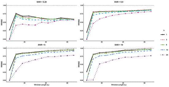
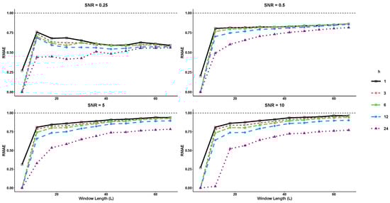
where the noise term ${\epsilon }_t$ is generated from a normal distribution at varying levels of signal-to-noise ratio (SNR). In this example, both basic SSA and SSD methods are compared using a rank value of $r=5$ for forecasting horizons of $h=1,3,6,12,$ and 24 steps ahead. The R-SSD method outperforms the basic R-SSA method in terms of forecasting accuracy across all window lengths (L) and SNR levels tested, as shown in Figure 1 and Figure 2. For nearly all forecast horizons h, the values of RRMSE and RMAE are less than 1, indicating that the R-SSD method provides more accurate predictions than the R-SSA method. The accuracy is consistent across different metrics, with the lowest RRMSE and RMAE values occurring at the lowest window length level ($L=6$) for all SNR levels when $h=12$ and 24. Overall, the results suggest that the R-SSD method is superior to the R-SSA method in providing accurate predictions.

Example 2. 

Example 2 involves an exponential series with two different frequencies as follows:

$$y_t=\left\{\begin{array}{c}exp({\alpha }_0+{\alpha }_{1}t)+cos(2\pi t/6)+{\epsilon }_t,1\le t\le 100\hfill \\ exp({\alpha }_0+{\alpha }_{1}t)+cos(5\pi t/6)+{\epsilon }_t,101\le t\le 200\hfill \end{array}\right.$$

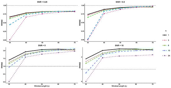
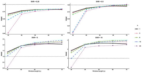
where the term ${\epsilon }_t$ represents the noise generated from a normal distribution at various levels of signal-to-noise ratio (SNR). In this study, both basic SSA and SSD methods use a rank of 25 for the trajectory matrix of the time series, with ${\alpha }_0=0$ and ${\alpha }_1=0.01$. RRMSE and RMAE are computed for various forecast horizons ($h=1,3,6,12$, and 24) and SNR levels. As shown in Figure 3 and Figure 4, RRMSE and RMAE increase as the forecast horizon decreases, but decrease significantly when $h=24$. The results indicate that the R-SSD method performs better as the value of L decreases. However, for higher SNR levels, the R-SSA method outperforms the R-SSD method for larger values of L. The lowest RRMSE and RMAE values are achieved when the window length and SNR are at their lowest values.

4.2. Real Data Analysis

In this section, we compare the forecasting performance of the proposed R-SSD method with the basic R-SSA method using real data from fruit fly (Drosophila melanogaster) embryos. The caudal protein in fruit fly embryos plays a crucial role in tail formation, acting as a transcription factor that regulates the expression of other genes by binding to specific DNA sequences. The caudal protein is expressed in the cells of the “tail bud”, which gives rise to the tail, and its activation triggers a gene expression cascade that controls cell division, differentiation, and migration, ultimately leading to tail formation. Mutations in the caudal gene can result in a loss of function of the protein, leading to defects in tail formation such as a short or absent tail, as well as other developmental defects related to segmentation. However, it is important to note that causality detection techniques, as demonstrated by previous studies, can be sensitive to noise [23,28,29,30]. Here, we analyze four gene expression profiles with varying lengths and dominant frequencies to demonstrate the importance of utilizing an accurate noise filtering method, such as SSD, for conducting reliable causality studies. To compare the forecasting performance of the R-SSA and R-SSD approaches, we provide

Table 1. RRMSE and RMAE analysis of Cad Profile ab2, $1/f_{max}=2$ with $r=16$.

Horizon	L = 20		L = 30		L = 50
	RRMSE	RMAE	RRMSE	RMAE	RRMSE	RMAE
1	0.96	0.96	1.02	1.02	1.12	1.12
3	0.86	0.91	1.03	1.05	1.13	1.16
6	0.78	0.80	0.96	1.02	1.09	1.19
12	0.59	0.62	0.86	0.92	1.11	1.22
24	0.17	0.21	0.59	0.67	1.00	1.09

,

Table 2. RRMSE and RMAE analysis for Cad profile ab18, $1/f_{max}=2$, with $r=14$.

Horizon	L = 20		L = 50		L = 80
	RRMSE	RMAE	RRMSE	RMAE	RRMSE	RMAE
1	0.82	0.82	1.27	1.27	1.14	1.14
3	0.88	0.86	1.15	1.21	1.01	1.07
6	0.91	0.92	1.17	1.26	1.03	1.10
12	0.90	0.91	1.23	1.31	1.08	1.17
24	0.84	0.86	1.25	1.36	1.16	1.31

,

Table 3. RRMSE and RMAE analysis of Cad Profile be11, $1/f_{max}=3$ with 3.

Horizon	L = 6		L = 18		L = 30
	RRMSE	RMAE	RRMSE	RMAE	RRMSE	RMAE
1	1.16	1.16	1.21	1.21	1.15	1.15
3	1.16	1.17	1.07	1.11	1.13	1.17
6	1.22	1.20	1.05	1.09	1.11	1.16
12	1.35	1.38	0.80	0.85	0.95	0.98
24	1.89	2.03	0.21	0.25	0.43	0.44

and

Table 4. RRMSE and RMAE analysis of Cad Profile ad14, $1/f_{max}=11$ with 5.

Horizon	L = 11		L = 88		L = 110
	RRMSE	RMAE	RRMSE	RMAE	RRMSE	RMAE
1	1.26	1.26	1.28	1.28	1.15	1.15
3	1.22	1.30	1.23	1.30	1.17	1.17
6	1.12	1.25	1.27	1.33	1.16	1.20
12	0.96	1.03	1.37	1.43	1.31	1.32
24	0.73	0.78	1.50	1.59	1.47	1.53

to summarize the obtained results for four different time classes: ab2, ab18, be11, ad14. These tables display the respective forecasting metrics, including RRMSE and RMAE, for each time class, enabling a comprehensive comparison between the two methods. For each dataset, we considered the first 80% of observations as the training sample and the remaining 20% as the test sample. The number of leading eigenvalues $\left(r\right)$ for reconstructing and forecasting the time series was selected based on the rank of the corresponding trajectory matrix. Additionally, the dominant frequency of the data ($1/f_{max}$) was calculated for each dataset, and the window length was chosen as a multiple of $1/f_{max}$ and less than $N/2$. After selecting the appropriate L and r, we utilized the observations from the training set to forecast the test sample data and calculate the RRMSE and RMAE criteria for different h step-ahead recurrent forecasts, using Equations (4) and (5).

Based on the results presented in Table 1, it is evident that there is a discernible difference in the RRMSE and RMAE values obtained using the R-SSA and R-SSD methods for $L=20,30,$ and 50. The performance metrics show contrasting outcomes for these window lengths, indicating that the choice of method can significantly impact the forecasting accuracy.

Table 2 shows the RRMSE and RMAE values obtained by each model for the cad profile ab18. As indicated in the table, the R-SSD method achieves a significant reduction in both RRMSE and RMAE values for $L=20$, which suggests that it generally provides better signal extraction and forecast results compared to the R-SSA model for this window length. Additionally, for $L=50$ and 80, the accuracy of the two methods is similar, indicating that the R-SSD method can be preferable for smaller window lengths.

Table 3 summarizes the results of RRMSE and RMAE for the cad profile be11. The findings indicate that the R-SSD method outperforms the R-SSA method, particularly for $L=18$ and 30 and horizons $h=12$ and 24. Furthermore, a closer examination of the table reveals that the highest accuracy is obtained when $L=18$ and $h=24$, as evidenced by the greatest reduction in both RRMSE and RMAE values.

Additionally, the forecasting methods R-SSD and R-SSA were evaluated for statistical significance using the non-parametric two-sample Wilcoxon test and the Kolmogorov–Smirnov Predictive Accuracy (KSPA) test. The results show a statistically significant difference between the two methods, with R-SSD forecasts having smaller errors than R-SSA forecasts with 95% confidence based on the one-sided KSPA test. The two-sided KSPA test further supports the significant differences between the two methods with 95% confidence, and these findings are consistent across different embryos and L values, especially for h = 24. These results demonstrate the superior accuracy of the R-SSD method and highlight the importance of utilizing an accurate noise filtering method such as SSD for precise causality studies. The Wilcoxon test also confirms the significant differences between the two methods for all tested embryos and L values, with p-values less than 0.05.

5. Discussion

In this paper, we introduced a new forecasting method called Recurrent Singular Spectrum Decomposition (R-SSD), which improves upon the standard R-SSA method by enhancing the identification of fluctuation content and enabling a fully data-driven selection of window length and principal components for reconstructing component series based on dominant frequency periods. The results were evaluated using the non-parametric two-sample Wilcoxon test and RRMSE/RMAE criteria, which demonstrated the superiority of R-SSD over basic R-SSA in the majority of cases for various window lengths and forecasting horizons. KSPA tests confirmed the ability of R-SSD to obtain significant components for accurate forecasting of new data points. In summary, the proposed R-SSD method with its improved trajectory matrix definition and window length selection shows promising results in time series forecasting. Overall, the R-SSD method offers a viable alternative to the standard R-SSA method and could lead to improved forecasting accuracy in a wide range of applications. Further research and investigation into the R-SSD method’s performance under different scenarios and datasets may be valuable for its continued development and potential adoption in practical settings.

References

- Broomhead, D.S.; King, G. Extracting qualitative dynamics from experimental data. Phys. D Nonlinear Phenom. 1989, 20, 217–236. [Google Scholar] [CrossRef]
- Hassani, H.; Ghodsi, Z.; Silva, E.; Heravi, S. From nature to maths: Improving forecasting performance in subspace-based methods using genetics Colonial Theory. Digit. Signal Process. 2016, 51, 101–109. [Google Scholar] [CrossRef]
- Gong, Y.; Song, Z.; He, M.; Gong, W.; Ren, F. Precursory waves and eigenfrequencies identified from acoustic emission data based on Singular Spectrum Analysis and laboratory rock-burst experiments. Int. J. Rock Mech. Min. Sci. 2017, 91, 155–169. [Google Scholar] [CrossRef]
- Yu, C.; Li, Y.; Zhang, M. An improved Wavelet Transform using Singular Spectrum Analysis for wind speed forecasting based on Elman Neural Network. Energy Convers. Manag. 2017, 148, 895–904. [Google Scholar] [CrossRef]
- Rahman Khan, M.R.; Poskitt, D.S. Forecasting stochastic processes using singular spectrum analysis: Aspects of the theory and application. Int. J. Forecast. 2017, 33, 199–213. [Google Scholar] [CrossRef]
- Heravi, S.; Osborn, D.R.; Birchenhall, C.R. Linear versus neural network forecasts for European industrial production series. Int. J. Forecast. 2004, 20, 435–446. [Google Scholar] [CrossRef]
- Lai, L.; Guo, K. The performance of one belt and one road exchange rate: Based on improved singular spectrum analysis. Phys. A Stat. Mech. Its Appl. 2017, 483, 299–308. [Google Scholar] [CrossRef]
- Hassani, H.; Yeganegi, M.; Khan, A.; Silva, E. The Effect of Data Transformation on Singular Spectrum Analysis for Forecasting. Signals 2020, 1, 4–25. [Google Scholar] [CrossRef]
- Hassani, H.; Silva, E.S.; Antonakakis, N.; Filis, G.; Gupta, R. Forecasting accuracy evaluation of tourist arrivals. Ann. Tour. Res. 2017, 63, 112–127. [Google Scholar] [CrossRef]
- Movahedifar, M.; Hassani, H.; Yarmohammadi, M.; Kalantari, M.; Gupta, R. A robust approach for outlier imputation: Singular spectrum decomposition. Commun. Stat. Case Stud. Data Anal. Appl. 2021, 8, 234–250. [Google Scholar] [CrossRef]
- Chao, S.; Loh, C. Application of singular spectrum analysis to structural monitoring and damage diagnosis of bridges. Struct. Infrastruct. Eng. 2014, 10, 708–727. [Google Scholar] [CrossRef]
- Chen, Q.; van Dam, T.; Sneeuw, N.; Collilieux, X.; Weigelt, M.; Rebischung, P. Singular spectrum analysis for modeling seasonal signals from GPS time series. J. Geodyn. 2013, 72, 25–35. [Google Scholar] [CrossRef]
- Hassani, H.; Webster, A.; Silva, E.; Heravi, S. Forecasting U.S. Tourist arrivals using optimal Singular Spectrum Analysis. Tour. Manag. 2015, 46, 322–335. [Google Scholar] [CrossRef]
- Hutny, A.; Warzecha, M.; Derda, W.; Wieczorek, P. Segregation of Elements in Continuous Cast Carbon Steel Billets Designated for Long Products. Arch. Metall. Mater. 2016, 61, 2037–2042. [Google Scholar] [CrossRef]
- Liu, K.; Law, S.; Xia, Y.; Zhu, X.Q. Singular spectrum analysis for enhancing the sensitivity in structural damage detection. J. Sound Vib. 2014, 333, 392–417. [Google Scholar] [CrossRef]
- Muruganatham, B.; Sanjith, M.A.; Kumar, B.; Murty, S.A.V.; Swaminathan, P. Roller element bearing fault diagnosis using singular spectrum analysis. Mech. Syst. Signal Process. 2013, 35, 150–166. [Google Scholar] [CrossRef]
- Sanei, S.; Hassani, H. Singular Spectrum Analysis of Biomedical Signals; CRC Press: Boca Raton, FL, USA, 2015. [Google Scholar]
- Movahedifar, M.; Yarmohammadi, M.; Hassani, H. Bicoid signal extraction: Another powerful approach. Math. Biosci. 2018, 303, 52–61. [Google Scholar] [CrossRef]
- Hiemstra, C.; Jones, J.D. Testing for Linear and Nonlinear Granger Causality in the Stock Price- Volume Relation. J. Financ. 1994, 49, 1639–1664. [Google Scholar]
- Ancona, N.; Marinazzo, D.; Stramaglia, S. Radial basis function approach to nonlinear Granger causality of time series. Phys. Rev. E Stat. Nonlinear Soft Matter Phys. 2004, 70, 056221. [Google Scholar] [CrossRef]
- Bonizzi, P.; Karel, J.; Meste, O.; Peeters, R. Singular Spectrum Decomposition: A new method for time series decomposition. Adv. Adapt. Data Anal. 2014, 6, 1450011. [Google Scholar] [CrossRef]
- Hassani, H. Singular Spectrum Analysis: Methodology and Comparison. J. Data Sci. 2007, 5, 239–257. [Google Scholar] [CrossRef] [PubMed]
- Golyandina, N.; Korobeynikov, A.; Zhigljavsky, A. Singular Spectrum Analysis with R; Springer: Berlin/Heidelberg, Germany, 2018. [Google Scholar] [CrossRef]
- Golyandina, N.; Nekrutkin, V.; Zhigljavsky, A.A. Analysis of Time Series Structure: SSA and Related Techniques, 1st ed.; Chapman and Hall/CRC: Boca Raton, FL, USA, 2001. [Google Scholar] [CrossRef]
- Golyandina, N.; Zhigljavsky, A. Singular Spectrum Analysis for Time Series; Springer: Berlin/Heidelberg, Germany, 2013. [Google Scholar]
- Vautard, R.; Yiou, P.; Ghil, M. Singular-spectrum analysis: A toolkit for short, noisy chaotic signals. Phys. D Nonlinear Phenom. 1992, 58, 95–126. [Google Scholar] [CrossRef]
- Hassani, H.; Silva, E. A Kolmogorov–Smirnov Based Test for Comparing the Predictive Accuracy of Two Sets of Forecasts. Econometrics 2015, 3, 590–609. [Google Scholar] [CrossRef]
- Vautard, R.; Ghil, M. Singular spectrum analysis in nonlinear dynamics, with applications to paleoclimatic time series. Phys. D Nonlinear Phenom. 1989, 35, 395–424. [Google Scholar] [CrossRef]
- Zou, C.; Feng, J. Granger causality vs. dynamic Bayesian network inference: A comparative study. BMC Bioinform. 2009, 10, 122. [Google Scholar]
- Golyandina, N.E.; Holloway, D.M.; Lopes, F.J.; Spirov, A.V.; Spirova, E.N.; Usevich, K.D. Measuring gene expression noise in early Drosophila embryos: Nucleus-to-nucleus variability. Procedia Comput. Sci. 2012, 9, 373–382. [Google Scholar] [CrossRef]
Disclaimer/Publisher’s Note: The statements, opinions and data contained in all publications are solely those of the individual author(s) and contributor(s) and not of MDPI and/or the editor(s). MDPI and/or the editor(s) disclaim responsibility for any injury to people or property resulting from any ideas, methods, instructions or products referred to in the content. |
© 2023 by the authors. Licensee MDPI, Basel, Switzerland. This article is an open access article distributed under the terms and conditions of the Creative Commons Attribution (CC BY) license (https://creativecommons.org/licenses/by/4.0/).