Proceeding Paper

Slope Entropy Characterisation: Adding Another Interval Parameter to the Original Method †

Department of System Informatics and Computers, Universitat Politècnica de València, 03801 Alcoy, Spain
*
Author to whom correspondence should be addressed.
Presented at the 9th International Conference on Time Series and Forecasting, Gran Canaria, Spain, 12–14 July 2023.
Eng. Proc. 2023, 39(1), 67; https://doi.org/10.3390/engproc2023039067
Published: 7 July 2023
(This article belongs to the Proceedings of The 9th International Conference on Time Series and Forecasting)

Abstract

:
Slope Entropy (SlpEn) is a recently proposed time series entropy estimation method for classification. This method has yielded better results than other similar methods in all the published studies so far. It is based on a signal-gradient thresholding scheme using two parameters, δ and γ , in addition to the usual embedded dimension parameter m. In this work, we investigated the possibility of adding one thresholding parameter more, termed θ , and we compared the original method to the new one. The experiment results showed a small improvement using the new method in terms of classification accuracy. However, the temporal cost increased significantly and therefore we concluded it is not worth the extra effort unless maximum accuracy is of utmost importance.

1. Introduction

Entropy estimation methods are very popular among scientists for extracting part of the possible hidden information present in a time series. These methods calculate the relative frequency of a set of numerical or symbolic subsequences. Many scientific fields have benefited from the high segmentation power of these methods. For example, they have been widely used in biomedicine to classify electroencephalograms, time series of electrocardiogram-RR, body temperature, and actigraph records, among many others. Each of the current entropy calculation methods has its strengths and weaknesses.
In this work, we investigated the effect of adding more gradient quantisation intervals to the recently proposed Slope Entropy (SlpEn) method on signal classification accuracy [1,2]. This method is based on assigning symbols to intervals of slopes between consecutive samples of time series [2].
In the general method, the δ and γ thresholds are responsible for labelling a slope (difference between two time series consecutive samples) as low, high, or flat (tie). If it is below δ , it is classified as tie. If it is between δ and γ , the slope is considered low. Otherwise, it is high.
The analysis was carried out as a comparative study. Many datasets with different signal types were employed to understand the impact of using a new additional gradient parameter in SlpEn. A grid search assessed the behaviour of all the datasets with different values of the input parameters to optimise them, see δ < γ and γ < θ in the new SlpEn variation.
The results obtained confirmed that adding a new parameter resulted in a small improvement in the classification accuracy. Specifically, the highest increment achieved using the new variation was 3 % higher, at most. However, the execution time was a lot longer than for the original SlpEn method due to the nested resulting additional combinations of δ , γ , and θ values in the grid search.
The structure of the paper is as follows. In Section 2, we present the datasets used in the experiments, a review of SlpEn, the proposed variation method, and the classification process. In Section 3, we report all the results. In Section 4, we provide an interpretation and analysis of all the results. Finally, we summarise our conclusions in the last section.

2. Methods

2.1. Datasets

The experimental dataset comprises several types of time series with different characteristics in terms of bandwidth, length, and regularity. All of them are publicly available, and many of the databases from which they have been extracted have already been used in similar works, serving as a reference for result comparison. The datasets are (two classes are used from each one):
The Bern–Barcelona database [3]: A set of electroencephalographic records.
The Fantasia database [4]: A set of electrocardiographic records of R-R intervals.
The Ford A dataset [5]: A set of records obtained from industrial processes.
The House Twenty dataset [6]: A set of records obtained from the electricity consumption of 20 households in the UK.
The PAF prediction dataset [7]: A set of electrocardiographic records of R-R intervals.
The Worms two class dataset [8,9]: A set of records obtained from the movement of genetically modified worms.
The Bonn EEG dataset [10]: A set of electroencephalographic records.

2.2. SlpEn

SlpEn applies the general expression of Shannon entropy to the estimated probabilities of a set of symbols. These symbols are assigned based on a range of differences between consecutive samples of subsequences extracted from a time series, X = { x 0 , x 1 , x 2 , , x N 1 } . These symbols are generically obtained from x i x i 1 , with the thresholds defined by the two parameters mentioned above: δ and γ [2]. Typically, δ is assigned a value of 0.001 .
In the standard method, symbols +2, + 1 , 0, −1, and −2 are assigned according to the range in which the differences are located. This process is graphically represented in Figure 1.
For each subsequence of length m, the corresponding symbol string is generated, and a histogram is constructed with the number of occurrences of each pattern. Finally, Shannon entropy is calculated on this histogram, as previously discussed.

2.3. Modified SlpEn Using an Additional Gradient Interval

In the original method, symbols are assigned based on the difference between two consecutive values. If the value x i x i 1 < δ , the symbol 0 is assigned and the slope is considered a tie. If the value x i x i 1 > δ and x i x i 1 > γ or x i x i 1 < δ and x i x i 1 < γ , the symbol 1 or 1 is assigned, and the slope is considered low. The last symbols assigned are 2 and 2 , respectively, when the values x i x i 1 > γ or x i x i 1 < γ , indicating that the slope is high.
The proposed modified SlpEn splits the symbols into three levels instead, including ties. Therefore, the assignment of symbols is now as follows.
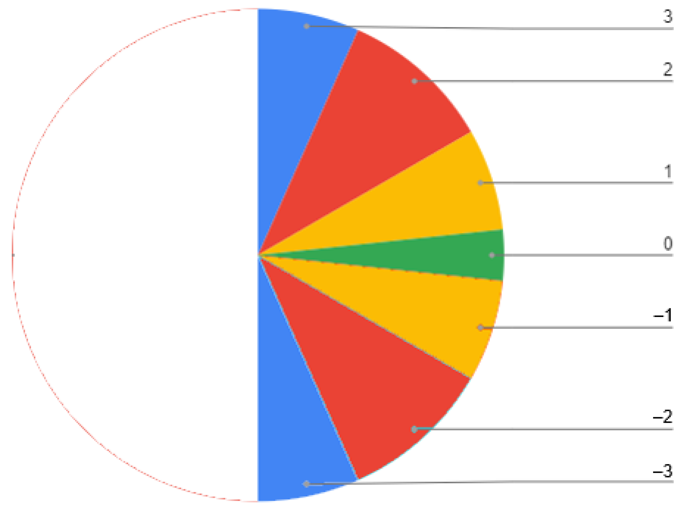
If x i > x i 1 + θ (maximum difference with respect to the parameter θ ), the symbol assigned is +3, indicating a large positive slope.
If x i > x i 1 + γ and x i x i 1 + θ indicating a medium positive slope, the symbol assigned is +2.
If x i > x i 1 + δ and x i x i 1 + γ (below γ ), an area that can be considered low from the point of view of positive slopes, the symbol assigned is +1.
In the region close to a gradient or slope of 0, when | x i x i 1 | γ , the symbol assigned is 0. This area represents ties or equal values, which can create ambiguities in other metrics.
If x i < x i 1 δ and x i x i 1 γ (above the 45 angle when γ = 1 and below the 0 slope zone), the resulting symbol is −1. SlpEn uses a symmetric quantization, but an asymmetric one could be used in future studies.
If x i < x i 1 γ and x i x i 1 + is assigned as symbol −2, representing the average negative value.
Finally, if x i < x i 1 θ (maximum negative difference with respect to the parameter θ ), the symbol assigned is −3, indicating a large negative slope.
So, instead of having −2, −1, 0, 1, and 2, we now have −3, −2, −1, 0, 1, 2, and 3, as shown in Figure 2.

2.4. Classification Scheme

Using the experimental datasets described earlier, the optimal value of SlpEn that maximised the accuracy of classifying records was calculated using the symmetric strategy represented in Figure 1 and Figure 2. Classification accuracy was defined as the percentage or ratio of time series correctly classified with respect to the total number of series in an experimental dataset.
This process was repeated using a three-parameter distribution of regions as in Figure 2. Now, in addition to having a specific value of γ , a higher value of θ was required. On the negative slopes region, θ is lower than γ , following the relationship γ < θ and γ > θ .
A time series classification analysis was carried out, comparing accuracy between the original SlpEn and the new proposed SlpEn variation. A grid search was conducted using the described databases in Section 2.1 to find the optimal input parameter combination that yielded maximum accuracy in each case.
For the baseline SlopEn method, we varied the parameter m within the range 3 to 9, the δ parameter from 0 to δ , and γ from δ to 1.5 . When using the additional parameter, θ varied from γ to 1.5 . The threshold used for classification was obtained from the ROC curve of the process [11]. Specifically, the point on the curve closest to ( 1 , 0 ) was used.

3. Experiments and Results

The experiments results showed a small improvement using the newly proposed method. Specifically, the proposed SlpEn variation exhibited small improvements of around 3 % in classification accuracy after using a grid search. Table 1 presents a report of the highest values of accuracy obtained with both SlpEn methods. However, the modified SlpEn is far more time consuming than the original SlpEn.

4. Discussion

The highest reported accuracy was for Fantasia, which improved by 3 % from 86 % to 89 % . PAF prediction and Bern–Barcelona both increased by 2 % , from 79 % to 81 % and from 81 % to 83 % , respectively. Ford A, House Twenty, Worms two class, and Bonn EEG datasets maintained the same accuracy, at 94 % , 97 % , 72 % , and 95 % , respectively.
Dividing the gradient into three or five levels does not seem to have a clear impact on classification performance. Therefore, adding more parameters to SlpEn is not advisable considering the amount of time consumed to achieve the small accuracy gains.

5. Conclusions

In this work, we presented a comparative study using different time series datasets to understand the impact of adding a new thresholding parameter to SlpEn. We introduced the parameter θ , and added it to δ and γ , expanding the symbolic intervals from 2 , 1 , 0 , 1 , and 2 to 3 , 2 , 1 , 0 , 1 , 2 , and 3 . The results confirmed that the new method achieved a minor improvement of 3 % , but at the expense of a significant processing time increase. Therefore, we do not recommend adding a new thresholding parameter due to the diminishing return achievable, unless a minor classification improvement is critical (for instance, in medical diagnosis applications).

Author Contributions

M.K. implemented the algorithms and carried out the experiments, and also wrote the initial version of the paper and prepared the presentation. D.C.-F. devised the idea and objectives of the study, the methodology, and reviewed the paper and the presentation. All authors have read and agreed to the published version of the manuscript.

Funding

This research received no external funding.

Institutional Review Board Statement

Not applicable.

Informed Consent Statement

Not applicable.

Data Availability Statement

All the data used in the experiments is publicly available at the sites included in the bibliographic references.

Conflicts of Interest

The authors declare no conflict of interest.

References

  1. Kouka, M.; Cuesta-Frau, D. Slope Entropy Characterisation: The Role of the δ Parameter. Entropy 2022, 24, 1456. [Google Scholar] [CrossRef]
  2. Cuesta-Frau, D. Slope entropy: A new time series complexity estimator based on both symbolic patterns and amplitude information. Entropy 2019, 21, 1167. [Google Scholar] [CrossRef] [Green Version]
  3. Andrzejak, R.G.; Schindler, K.; Rummel, C. Nonrandomness, nonlinear dependence, and nonstationarity of electroencephalographic recordings from epilepsy patients. Phys. Rev. E 2012, 86, 046206. [Google Scholar] [CrossRef] [PubMed] [Green Version]
  4. Iyengar, N.; Peng, C.K.; Morin, R.; Goldberger, A.L.; Lipsitz, L.A. Age-related alterations in the fractal scaling of cardiac interbeat interval dynamics. Am. J. Physiol. Regul. Integr. Comp. Physiol. 1996, 271, R1078–R1084. [Google Scholar] [CrossRef] [PubMed] [Green Version]
  5. FordA Description. Available online: http://www.timeseriesclassification.com/description.php?Dataset=FordA (accessed on 7 March 2023).
  6. HouseTwenty. Available online: http://www.timeseriesclassification.com/description.php?Dataset=HouseTwenty (accessed on 7 March 2023).
  7. Dean, M.E. Prefiltering for Improved Unknown and Known Source Correlation Detection of Broadband Oscillatory Transients and Predicting the Onset of Paroxysmal Atrial Fibrillation Using Feature Extraction and a Hamming Neural Network; University of New Orleans: New Orleans, LA, USA, 2003. [Google Scholar]
  8. WormsTwoClass. Available online: https://www.timeseriesclassification.com/description.php?Dataset=WormsTwoClass (accessed on 7 March 2023).
  9. Yemini, E.; Jucikas, T.; Grundy, L.J.; Brown, A.E.; Schafer, W.R. A database of caenorhabditis elegans behavioral phenotypes. Nat. Methods 2013, 10, 877–879. [Google Scholar] [CrossRef] [PubMed] [Green Version]
  10. Tsipouras, M.G. Spectral information of EEG signals with respect to epilepsy classification. Eurasip J. Adv. Signal Process. 2019, 2019, 10. [Google Scholar] [CrossRef] [Green Version]
  11. Hand, D.J.; Till, R.J. A simple generalisation of the area under the ROC curve for multiple class classification problems. Mach. Learn. 2001, 45, 171–186. [Google Scholar] [CrossRef]
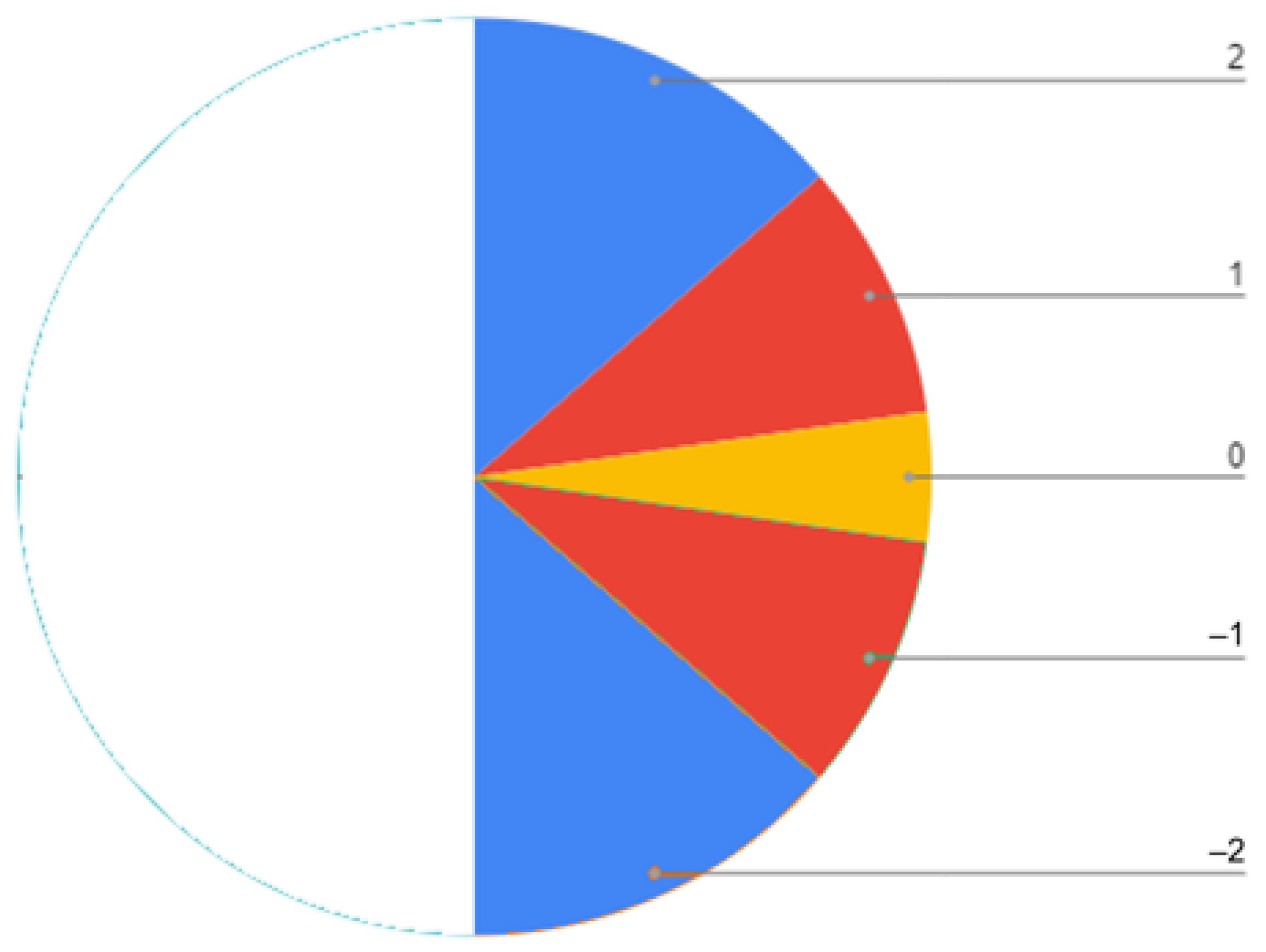
Figure 1. Graphical representation of the calculation of symbols used in SlpEn based on the thresholds γ and δ .
Engproc 39 00067 g001
Figure 2. Graphical representation of the calculation of symbols used in SlpEn based on the thresholds γ , δ , and θ .
Engproc 39 00067 g002
Table 1. A comparative study between original SlpEn and modified SlpEn.
Classification Accuracy
DatasetsOriginal SlpEnModified SlpEn
The Bern–Barcelona 79 % 81 %
The Fantasia 86 % 89 %
The Ford A 94 % 94 %
The House Twenty 97 % 97 %
The PAF prediction 81 % 83 %
The Worms two class 72 % 72 %
The Bonn EEG dataset 95 % 95 %
Disclaimer/Publisher’s Note: The statements, opinions and data contained in all publications are solely those of the individual author(s) and contributor(s) and not of MDPI and/or the editor(s). MDPI and/or the editor(s) disclaim responsibility for any injury to people or property resulting from any ideas, methods, instructions or products referred to in the content.