Abstract
Transfer learning has not been widely explored with time series. However, it could boost the application and performance of deep learning models for predicting macroeconomic time series with few observations, like monthly variables. In this study, we propose to generate a forecast of five macroeconomic variables using deep learning and transfer learning. The models were evaluated with cross-validation on a rolling basis and the metric MAPE. According to the results, deep learning models with transfer learning tend to perform better than deep learning models without transfer learning and other machine learning models. The difference between statistical models and transfer learning models tends to be small. Although, in some series, the statistical models had a slight advantage in terms of the performance metric, the results are promising for the application of transfer learning to macroeconomic time series.
1. Introduction
It is necessary to generate forecasts of macroeconomic variables for national economic policy and financial decision-making [1,2]. For this reason, Centrals Banks, international institutions, and economic research bodies allocate time and resources to generate accurate forecasts [3,4]. The prediction of macroeconomic and financial variables is regarded as one of the most challenging applications of modern time series forecasting [5].
In recent years, deep learning models have gained relevance in the time series field because they have shown high prediction capacity in several tasks, like the forecasting of electricity consumption [6], weather conditions [7] and other tasks. Nevertheless, its implementation in macroeconomic forecasts has been scarce [8,9,10,11]. A possible reason is that deep learning performs better with large datasets and some macroeconomic variables have a low number of observations [4], especially monthly or quarterly time series. For example, 30 years of observations would only amount to 360 observations for a monthly time series. This issue is still more relevant in some emerging countries where it is difficult to find a long history of information [11].
An alternative to building deep learning models with short time series is to train a model using a handful of diverse time series. Then, the pre-trained model can be used for transfer learning with the target time series. Transfer learning has not been widely explored with time series; however, there is evidence of good results [12,13,14].
In this study, we applied transfer learning with monthly macroeconomic variables to analyze the performance of deep learning models for forecasting macroeconomic time series. Our main contributions are the following:
- ✓
- As far as we know, this is the first study that explores and proposes the generation of pre-trained models that can be used with transfer learning to make predictions in any country using monthly macroeconomic variables.
- ✓
- Some studies compare the performance of several models with macroeconomic variables; however, as far as we know, this is the first that makes a benchmark between deep learning, statistical, and machine learning models.
- ✓
- This study compares the application of deep learning models without transfer learning, as economic researchers tend to do, and the application of deep learning models with transfer learning.
Our results suggest that the latter procedure is the better practice. Therefore, the study provides findings that can be relevant to economic and financial forecast research.
2. Deep Learning Applied to Macroeconomic Variables Forecast
Some studies have used deep learning to generate forecast models for macroeconomic variables such as exchange rate [5], inflation [2], unemployment rate [15], GDP [16], interest rate [17], and exports [11]. The periodicity of the time series used is diverse, and ranges from daily to annual. When the periodicity is less frequent, such as monthly and quarterly, the time series are short; however, deep learning models without transfer learning have shown good results e.g., [4,5]. For this reason, we also used deep learning without transfer learning.
The deep learning architectures for macroeconomic predictions tend to be based on Long Short-Term Memory, which is expected, because, unlike other networks, the LSTM takes into account the sequential pattern of the time series. Some researchers have used simple LSTM [18] or LSTM encoder–decoder [9], and others have created their own architectures. For example, in [19] they created a model named DC-LSTM, which is based on a first layer using two LSTM models to learn the features. In the second layer, a coupled LSTM is built on the features learned from the first layer. Then, the learned features are fed into a fully connected layer to make the forecast. For their part, in [20] they generated an ensemble of LSTM using bagging to predict the daily exchange rate. For the prediction, they computed the median value of the k replicas. Besides LSTM, other recurrent neuronal networks have been used as a gated recurrent unit [15]. Some researchers have used non-recurrent networks such as Fully Connected Architecture, Convolutional Neuronal Networks with residual connections [21], Neural Network Autoregression (NNAR) models [10], multilayer perceptron (MLP) [15], and stacked autoencoders [8].
The models are trained using different inputs. Some models only use the lagged values of the time series as an input to the neural network e.g., [10,18], while others also use the lagged values of other time series e.g., [2,4]. A particular case is the model of [17], who incorporated Twitter sentiment related to multiple events happening around the globe into interest rate prediction.
Concerning macroeconomic prediction performance, deep learning has shown good results. For example, [5] found that LSTM outperformed VAR and SVM for predicting the monthly USD–INR foreign exchange rate. In [8] they concluded that stacked autoencoders achieve more accurate results than support vector machines for predicting the 0 daily EUR–USD exchange rate. In [2] they found that LSTM had the best performance for the inflation prediction of more than one month compared to random forests, extreme gradient boosting, and k-nearest neighbors. According to [11], the deep learning approach showed better prediction powers than conventional econometric approaches such as VECM.
3. Method
3.1. Macroeconomic Time Series
Five economic time series variables from five countries were chosen for the analysis. The variables were: Consumer Price Index (CPI), Industrial Production Index (IPI), Value of Exports in US Dollars (TVE), Average Monthly Exchange Rates of domestic Currency per US Dollar (ER), and Producer Price Index (PPI). The countries analyzed were Costa Rica (CR), the United States (UE), the United Kingdom (UK), South Korea (SR), and Bulgaria (BU). In the case of the United States, we did not analyze domestic currency. Thus, 24 time series were used.
3.2. Datasets
Three datasets were built and used: (a) Dataset with the 24 target time series that were taken from the International Monetary Fund in May 2022; (b) Dataset with the economic variables mentioned before, from the countries shown by the FMI web page in May 2022 (https://data.imf.org/?sk=388DFA60-1D26-4ADE-B505-A05A558D9A42&sId=1479329132316, accessed on 22 May 2022), except for the countries used as the target. We deleted time series that did not show variability or had missing values. This dataset had 515-time series, and was named the macroeconomic dataset; (c) Dataset with 1000 time series taken randomly from the M4 competition [22]. This was named the M4 subsample. The last two datasets were built to generate the pre-trained models used for transfer learning.
3.3. Models
We analyzed five types of models:
- ✓
- Three statistical models (St): Auto Arima (arima), ETS (ets), and Theta (theta);
- ✓
- Machine learning models (Ml): Support vector regression (svr), random forest (rf) and XGBoost (xgb);
- ✓
- Deep learning models without transfer learning (Dl/wh): Long short-term memory (lstm), temporal convolutional network (tcn), convolutional neuronal network (cnn);
- ✓
- First proposal of deep learning with transfer Learning (Dl/t_M4). We applied the same deep learning models mentioned previously, but in this case, the models were trained with the 1000 time series concatenated from the M4 subsample dataset. The concatenation was in the input and output. For example, for the prediction of the next three months based on the previous twelve months, the all-time series was transformed into a matrix of k rows and fifteen columns; then, the matrices were concatenated to obtain the final dataset. Finally, when the models were trained, we used them to apply transfer learning for each of the target time series (the 24 time series)
- ✓
- The second proposal of deep learning with transfer learning (Dl/t). The methodology was like that of the previous models, but the models were trained using the macroeconomic dataset.
We generated models to predict three periods and twelve periods ahead. Two types of input sizes were proved in models B, C, D, and E. For the forecast horizon of three periods, we used the previous three periods and the previous twelve periods as input, and for the forecast horizon of twelve periods, we used the previous twelve periods and the previous fifteen periods. Finally, we only kept the model with the input size that achieved the best performance. The deep learning models were trained using the Adam optimizer and a stop criterion which consisted of stopping after two epochs without improvement in the validation sample’s loss function, which was the mean squared error. The hyperparameters of models B, C, D, and E and the architectures of the neuronal networks were defined in the training phase through Bayesian optimization. The search grid for the Bayesian optimization is in Table 1.

Table 1.
Search grid for the Bayesian optimization of Machine Learning Models.
The transfer learning for models D and E was realized in the last two layers of the model. The weights were updated using the target time series and a learning rate of 0.000005, which is less than that used in the training phase. A maximum of 75 epochs were set; however, the model could stop earlier if, after two epochs, there were no improvements in the mean square error of the validation sample.
3.4. Experimental Procedure
We used cross-validation on a rolling basis [23], also known as prequential or back testing, to evaluate the models’ performance and make comparisons between them. Figure 1 shows the general process. In the case of the machine learning and deep learning models, we split the training part into train and validation for the tuning. The performance metric MAPE was computed from the test sample in each of the ten replicas and then averaged to make the comparisons between models. In every replica, the test sample was the same as the model forecast horizon, either 3 or 12.
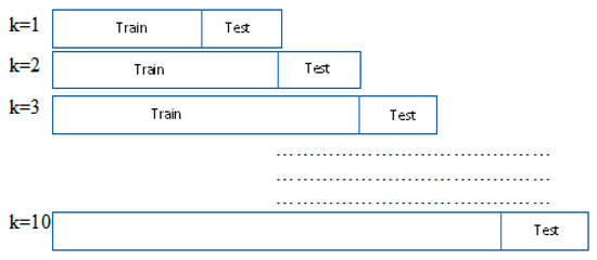
Figure 1.
Cross-validation on a rolling basis for the model’s evaluation.
4. Results
Table 2 and Table 3 show the average MAPE according to the model type for a horizon output of 3 and 12, respectively. The last two columns of each table present the best metric average of the transfer learning models and the best metric average for the rest of the models. The sky-blue color indicates which model has the lowest average metric, and the gray color indicates that there is no statistical difference between the type of models that the cells represent and the best model, using the Wilcoxon Sign Test with a p-value of 0.05.
Table 2.
Average MAPE for each kind of model when output horizon = 3.
Table 3.
Average MAPE for each kind of model when output horizon = 12.
We compare the deep learning models created from the M4 subsample dataset with the models created from the macroeconomic dataset to determine if the usage of a dataset more oriented to the domain of the target time series generates the best results. However, the performance metrics between both types of models were similar. Table 2 and Table 3 show that the MAPE was almost identical for most times series. Therefore, the M4 time series can be as valuable as the macroeconomic time series in generating pre-trained models for the variables analyzed in this study.
The results show that the deep learning models with transfer learning tended to perform better than deep learning models without transfer learning and other machine learning models for an output of 3 or 12. Recent studies have trained deep learning models directly on the economic monthly target time series e.g., [1,10,15]; however, our results suggest that there is a possibility that transfer learning could give the best performance.
The statistical models performed better in most time series than deep learning models with transfer learning, although the difference is not statistically significant for many time series. The differences between statistical and transfer learning models were smaller when the output was 12. For example, in 11 time series, there was a significant difference in the metric MAPE when the output was 3 (Table 2), and there was a significant difference in only four time series (Table 3) when the output was 12. Statistical models were not the best is all time series; there were time series for which the transfer learning models obtained the best results.
On the other hand, the results of the best specific models indicate that the best transfer learning model is mainly based on lstm for an output horizon of 3 and tcn for an output horizon of 12. The best of the other models was usually a statistical model for an output of 3 and 12. Although, in most time series, the statistical model had a slightly better value in terms of performance metric, the deep learning model has the advantage that it is simpler to make forecasts because only one model is required to predict the five variables in any country.
5. Conclusions
To our knowledge, this is the first study that analyses the application of transfer learning to macroeconomic monthly time series. Our conclusion is that transfer learning tends to perform better than the application of deep learning models without transfer learning and other machine learning models. The statistical models still provide better results in most cases, although their performance is mainly similar to that of transfer learning, and even in some series, the transfer learning showed better metrics values at a descriptive level. These findings are promising for applying transfer learning to macroeconomic time series which would simplify the generation of forecasts since, with a single pre-trained model, several economic variables can be predicted for different countries.
Additionally, there are different options to explore the generation of a model that improves the predictions of the statistical models. Future studies should apply transfer learning to other kinds of networks that have provided very positive results in natural language processing, such as transforms and seq2seq models. We only used the lags of the time series as input; however, it is relevant to analyze the performance of deep learning models when the lags of the own series and the information of external variables are received as input, which can be used for the prediction of specific macroeconomic variables. It could improve the performance of deep learning models that have shown the capacity to extract patterns from wide input arrays. Additionally, it is possible to explore the creation of a model trained with different datasets or create ensembles from different pre-trained models.
Author Contributions
Conceptualization, M.S. and L.-A.C.-V.; methodology, M.S. and L.-A.C.-V.; software, M.S.; validation, M.S.; formal analysis, M.S.; investigation, M.S. and L.-A.C.-V.; resources, M.S.; data curation, M.S.; writing—original draft preparation, M.S.; writing—review and editing, M.S. and L.-A.C.-V.; visualization, M.S.; supervision, M.S. All authors have read and agreed to the published version of the manuscript.
Funding
This research received no external funding.
Institutional Review Board Statement
Not applicable.
Informed Consent Statement
Not applicable.
Data Availability Statement
Macroeconomic datasets available at https://github.com/martin12cr/DatasetTL_macroeconomic, accessed on 22 May 2022.
Conflicts of Interest
The authors declare no conflict of interest.
References
- Vargas, A.R. Pronóstico del crecimiento trimestral de costa rica mediante modelos de frecuencia mixta. Rev. Cienc. Econ. 2014, 32, 189–226. [Google Scholar] [CrossRef][Green Version]
- Rodríguez-Vargas, A. Forecasting Costa Rican inflation with machine learning methods. Lat. Am. J. Central Bank. 2020, 1, 100012. [Google Scholar] [CrossRef]
- Aastveit, K.A.; McAlinn, K.; Nakajima, J.; West, M. Multivariate Bayesian Predictive Synthesis in Macroe-conomic Forecasting. J. Am. Stat. Assoc. 2019, 115, 1092–1110. [Google Scholar] [CrossRef]
- Jung, J.-K.; Patnam, M.; Ter-Martirosyan, A. An Algorithmic Crystal Ball: Forecasts-Based on Machine Learning. SSRN Electron. J. 2018, 2018, 1–35. [Google Scholar] [CrossRef]
- Kaushik, M.; Giri, A.K. Forecasting Foreign Exchange Rate: A Multivariate Comparative Analysis between Traditional Econometric, Contemporary Machine Learning & Deep Learning Techniques. arXiv 2020, arXiv:2002.10247. [Google Scholar]
- Mariano-Hernández, D.; Hernández-Callejo, L.; Solís, M.; Zorita-Lamadrid, A.; Duque-Perez, O.; Gonzalez-Morales, L.; Santos-García, F. A Data-Driven Forecasting Strategy to Predict Continuous Hourly Energy Demand in Smart Buildings. Appl. Sci. 2021, 11, 7886. [Google Scholar] [CrossRef]
- Hewage, P.; Behera, A.; Trovati, M.; Pereira, E.; Ghahremani, M.; Palmieri, F.; Liu, Y. Temporal convolutional neural (TCN) network for an effective weather forecasting using time-series data from the local weather station. Soft Comput. 2020, 24, 16453–16482. [Google Scholar] [CrossRef]
- Chen, J.; Zhao, C.; Liu, K.; Liang, J.; Wu, H.; Xu, S. Exchange Rate Forecasting Based on Deep Learning and NSGA-II Models. Comput. Intell. Neurosci. 2021, 2021, 2993870. [Google Scholar] [CrossRef] [PubMed]
- Nguyen, H.T.; Nguyen, D.T. Transfer Learning for Macroeconomic Forecasting. In Proceedings of the 2020 7th NAFOSTED Conference on Information and Computer Science (NICS), Ho Chi Minh City, Vietnam, 26–27 November 2020; IEEE: Piscataway, NJ, USA, 2020; pp. 332–337. [Google Scholar] [CrossRef]
- Pratap, B.; Sengupta, S. Macroeconomic Forecasting in India: Does Machine Learning Hold the Key to Better Forecasts? In RBI Working Paper Series; Reserve Bank of India: Mumbai, India, 2019. [Google Scholar] [CrossRef]
- Kim, S. Macroeconomic and Financial Market Analyses and Predictions through Deep Learning. In Bank of Korea WP 2020-18. Available online: https://ssrn.com/abstract=3684936 (accessed on 25 November 2021).
- Solís, M.; Calvo-Valverde, L.-A. Performance of Deep Learning models with transfer learning for multiple-step-ahead forecasts in monthly time series. Intel. Artif. 2022, 25, 110–125. [Google Scholar] [CrossRef]
- Otović, E.; Njirjak, M.; Jozinović, D.; Mauša, G.; Michelini, A.; Štajduhar, I. Intra-domain and cross-domain transfer learning for time series data—How transferable are the features? Knowl.-Based Syst. 2022, 239, 107976. [Google Scholar] [CrossRef]
- Poghosyan, A.; Harutyunyan, A.; Grigoryan, N.; Pang, C.; Oganesyan, G.; Ghazaryan, S.; Hovhannisyan, N. An Enterprise Time Series Forecasting System for Cloud Applications Using Transfer Learning. Sensors 2021, 21, 1590. [Google Scholar] [CrossRef] [PubMed]
- Mulaudzi, R.; Ajoodha, R. Application of Deep Learning to Forecast the South African Unemployment Rate: A Multivariate Approach. In Proceedings of the 2020 IEEE Asia-Pacific Conference on Computer Science and Data Engineering (CSDE), Gold Coast, Australia, 16–18 December 2020; IEEE: Piscataway, NJ, USA, 2020; pp. 1–6. [Google Scholar] [CrossRef]
- Longo, L.; Riccaboni, M.; Rungi, A. A neural network ensemble approach for GDP forecasting. J. Econ. Dyn. Control 2022, 134, 104278. [Google Scholar] [CrossRef]
- Yasir, M.; Afzal, S.; Latif, K.; Chaudhary, G.M.; Malik, N.Y.; Shahzad, F.; Song, O.-Y. An Efficient Deep Learning Based Model to Predict Interest Rate Using Twitter Sentiment. Sustainability 2020, 12, 1660. [Google Scholar] [CrossRef]
- Dodevski, A.; Koceska, N.; Koceski, S. Forecasting exchange rate between macedonian denar and euro using deep learning. J. Appl. Econ. Bus. 2018, 6, 50–61. [Google Scholar]
- Cao, W.; Zhu, W.; Wang, W.; Demazeau, Y.; Zhang, C. A Deep Coupled LSTM Approach for USD/CNY Exchange Rate Forecasting. IEEE Intell. Syst. 2020, 35, 43–53. [Google Scholar] [CrossRef]
- Sun, S.; Wang, S.; Wei, Y. A new ensemble deep learning approach for exchange rates forecasting and trading. Adv. Eng. Informatics 2020, 46, 101160. [Google Scholar] [CrossRef]
- Cook, T.R.; Hall, A.S. Macroeconomic Indicator Forecasting with Deep Neural Networks. In Proceedings of the CARMA 2018—2nd International Conference on Advanced Research Methods and Analytics, Valencia, Spain, 12–13 July 2018. [Google Scholar] [CrossRef]
- M4 Team. M4 Competitor’s Guide: Prizes and Rules. 2018. Available online: https://www.m4.unic.ac.cy/wpcontent/uploads/2018/03/M4-CompetitorsGuide.pdf (accessed on 25 November 2021).
- Hu, M.Y.; Zhang, G.; Jiang, C.X.; Patuwo, B.E. A Cross-Validation Analysis of Neural Network Out-of-Sample Performance in Exchange Rate Forecasting. Decis. Sci. 1999, 30, 197–216. [Google Scholar] [CrossRef]

Disclaimer/Publisher’s Note: The statements, opinions and data contained in all publications are solely those of the individual author(s) and contributor(s) and not of MDPI and/or the editor(s). MDPI and/or the editor(s) disclaim responsibility for any injury to people or property resulting from any ideas, methods, instructions or products referred to in the content. |
© 2023 by the authors. Licensee MDPI, Basel, Switzerland. This article is an open access article distributed under the terms and conditions of the Creative Commons Attribution (CC BY) license (https://creativecommons.org/licenses/by/4.0/).