Combining Forecasts of Time Series with Complex Seasonality Using LSTM-Based Meta-Learning ^†

Abstract

In this paper, we propose a method for combining forecasts generated by different models based on long short-term memory (LSTM) ensemble learning. While typical approaches for combining forecasts involve simple averaging or linear combinations of individual forecasts, machine learning techniques enable more sophisticated methods of combining forecasts through meta-learning, leading to improved forecasting accuracy. LSTM’s recurrent architecture and internal states offer enhanced possibilities for combining forecasts by incorporating additional information from the recent past. We define various meta-learning variants for seasonal time series and evaluate the LSTM meta-learner on multiple forecasting problems, demonstrating its superior performance compared to simple averaging and linear regression.

1. Introduction

Real-world time series can exhibit various complex properties such as time-varying trends, multiple seasonal patterns, random fluctuations, and structural breaks. Given this complexity, it can be challenging to identify a single best model to accurately approximate the underlying data-generating process [1]. To address this issue, a common approach is to combine multiple forecasting models to capture the multiple drivers of the data-generating process and mitigate uncertainties regarding model form and parameter specification [2]. This approach, known as ensemble forecasting or combining forecasts, has been shown to be effective in improving the accuracy and reliability of time series forecasts. By combining forecasts, the aim is to take advantage of the strengths of multiple models and reduce the impact of their individual weaknesses.

There are several potential explanations for the strong performance of forecast combinations. Firstly, by combining forecasts, the resulting ensemble can capture a broader range of information and better handle the forecasting problem complexity. It can leverage the strengths of individual models, as each model may capture different aspects of the underlying data-generating process. Therefore, the resulting ensemble can incorporate partial and incompletely overlapping information, leading to improved accuracy and robustness. Secondly, in the presence of structural breaks and other instabilities, combining forecasts from models with different degrees of misspecification and adaptability can mitigate the problem. This is because individual models may perform well under certain conditions but poorly under others, and by combining them, the ensemble can better handle a range of potential scenarios [3]. Finally, forecast combinations can improve stability compared to using a single model, as the ensemble is less sensitive to the idiosyncrasies of individual models. This means that the resulting forecasts are less likely to be influenced by outliers or errors in individual models, leading to more reliable predictions.

In a classical way, by combining the predictions from multiple models, the resulting ensemble prediction can be thought of as an average of the individual predictions. The variance of the average of multiple independent random variables is typically lower than the variance of a single random variable, assuming that the individual predictions are diverse. Therefore, a key issue in ensemble learning is ensuring diversity among the individual models being combined. If the models are too similar, the ensemble may not be able to capture the full range of possible outcomes and may not improve predictive performance. In this work, we ensure high diversity among models by using non-interfering models with different operating principles and architectures, including statistical, machine learning (ML), and hybrid models (see Section 3.2).

A simple arithmetic average of forecasts based on equal weights is a popular and surprisingly robust combination rule, outperforming more complicated weighting schemes in many cases [4,5]. Other strategies, such as using the median, mode, trimmed means, and winsorized means, are also applied [6]. To differentiate weights assigned to individual models, linear regression can be used, where the vector of past observations is the response variable and the matrix of past individual forecasts is the predictor variable. Combination weights can be estimated using ordinary least squares. The weights can reflect individual models’ performance on historical data [7]. Time-varying weights can be used to improve forecasting ability in the presence of instabilities, and principal components regression can be used as a solution for multicollinearity [8]. Weights can also be derived from information criteria such as AIC [9].

Linear combination approaches assume a linear dependence between constituent forecasts and the variable of interest, and may not result in the best forecast, especially if the individual forecasts come from nonlinear models or if the true relationship between base forecasts and the target has a nonlinear form [10]. In contrast, ML models can combine the base forecasts nonlinearly using a stacking procedure.

Stacking is an ensemble ML algorithm that learns how to best combine predictions from multiple models, using the concept of meta-learning to boost forecasting accuracy beyond that achieved by the individual models. Neural networks (NNs) are often used in stacking to estimate the nonlinear mapping between the target value and its forecasts produced by multiple models [11]. The power of ensemble learning for forecasting was demonstrated in [12], where several meta-learning approaches were evaluated on a large and diverse set of time series data. Ensemble methods were found to provide a benefit in overall forecasting accuracy, with simple ensemble methods leading to good results on average. However, there was no single meta-learning method that was suitable for all time series.

The main contributions of this study can be summarized in the following three aspects:

• A meta-learning approach based on LSTM is proposed for combining forecasts. This approach incorporates past information accumulated in the internal states, improving accuracy, especially in cases where there is a temporal relationship between base forecasts for successive time points.
• Various meta-learning variants for time series with multiple seasonal patterns are proposed, such as the use of the full training set, including base forecasts for successive time points, and the use of selected training points that reflect the seasonal structure of the data.
• Extensive experiments are conducted on 35 time series with triple seasonality using 16 base models to validate the efficacy of the proposed approach. The experimental results demonstrate the high performance of the LSTM meta-learner and its potential to combine forecasts more accurately than simple averaging and linear regression methods.

The remainder of this work is structured as follows. Section 2 presents the proposed LSTM meta-model and introduces both the global and local meta-learning variants. Section 3 provides application examples for time series with complex seasonality and discusses the results obtained from the conducted experiments. Finally, in Section 4, we conclude our work by summarizing the key findings and contributions.

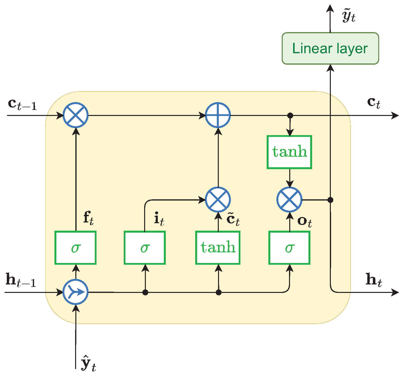
2. LSTM for Combining Forecasts

The problem of forecast combinations refers to the task of finding regression function f that aggregates the forecasts for time t produced by n forecasting models. The function can use all the available information up to time $t-h$, where h is a forecast horizon, but in this study, we limit this information to the base forecasts expressed by vector ${\widehat{\mathbf{y}}}_t=[{\widehat{y}}_{1,t},\dots ,{\widehat{y}}_{n,t}]$. The combined forecast is ${\tilde{y}}_t=f({\widehat{\mathbf{y}}}_t;{\mathit{\theta }}_t)$, where ${\mathit{\theta }}_t$ is a vector of meta-model parameters.

The model learns using training set $\mathrm{\Phi }={\{{\widehat{\mathbf{y}}}_{\tau },y_{\tau }\}}_{\tau \in \mathrm{\Xi }}$, where $y_{\tau }$ is a target value and $\mathrm{\Xi }$ is a set of selected time indexes from interval $T=1,\dots ,t-h$ (selection of this set is considered in Section 2.2).

The class of regression functions f encompasses both linear and nonlinear mappings, as well as series-specific and cross-learning mappings. In the latter approach, the parameters of the function are selected through a learning process over multiple time series, which enhances the generalization capability of the model. Furthermore, the parameters can either be static or time-varying throughout the forecasting horizon. To maximize the performance of the ensemble, we adopt an approach where we learn the meta-model parameters for each forecasting task individually, using a specific training set for each task (see Section 2.2).

2.1. LSTM Model

LSTM is a modern recurrent NN that incorporates gating mechanisms [13]. This NN architecture was specifically designed to handle sequential data and is capable of learning short and long-term relationships in time series [14]. LSTM is composed of recurrent cells that can maintain their internal states over time, i.e., cell state c and hidden state h. These cells are regulated by nonlinear gating mechanisms that control the flow of information within the cell, allowing it to adapt to the dynamics of the current process.

In our implementation, the LSTM network consists of two layers: the LSTM layer and the linear layer, see Figure 1. The LSTM layer is responsible for approximating temporal nonlinear dependencies in sequential data and generating state vectors. On the other hand, the linear layer converts hidden state vector h into the output value. The aggregation function implemented in the LSTM network can be written as:

$$f\left({\widehat{\mathbf{y}}}_t\right)={\mathbf{v}}^T{\mathbf{h}}_t\left({\widehat{\mathbf{y}}}_t\right)+v_0$$

(1)

$${\mathbf{h}}_t\left({\widehat{\mathbf{y}}}_t\right)=\mathrm{LSTM}({\widehat{\mathbf{y}}}_t,{\mathbf{c}}_{t-1},{\mathbf{h}}_{t-1};\mathbf{w})\in {\mathbb{R}}^m$$

(2)

where $\mathbf{w}$ and $\mathbf{v}$ are the weights of the LSTM and linear layers, respectively.

The number of nodes in each gate, m, is the most critical hyperparameter. It determines the amount of information stored in the states. For more intricate temporal relationships, a higher number of nodes is necessary.

In contrast to non-recurrent ML models such as feed-forward NNs, tree-based models, and support vector regression, to calculate output ${\tilde{y}}_t$, LSTM uses not only the information included in the base forecasts for time t, ${\widehat{\mathbf{y}}}_t$, but also in the base forecasts for previous time steps, $t-1,t-2,\dots$. This is achieved through states ${\mathbf{c}}_{t-1}$ and ${\mathbf{h}}_{t-1}$, which accumulate information from the past steps.

2.2. Meta-Learning Variants

The forecasting models generate forecasts for the successive time points $T=1,\dots ,t-h$. To obtain an ensemble forecast for time t, we can train the meta-model using all available data from the historical period, i.e., $\mathrm{\Xi }=T$, which is referred to as the global approach. Using this method, the model can utilize all available information to generate a forecast for the current time point.

In local learning, we restrict the training sequence to the last k points, i.e., $\mathrm{\Xi }=t-h-k,\dots ,t-h$, allowing the LSTM to model the relationship for the query pattern ${\widehat{\mathbf{y}}}_t$ based on the most recent sequence of length k. We refer to this approach as v1.

When ensembling seasonal time series, training the LSTM model on points from the same phase of the cycle as the forecasted point can improve forecast accuracy. In this approach, the training set consists of points $\mathrm{\Xi }=\{t-k{s}_1,t-(k-1)s_1,\dots ,t-s_1\}$, where $s_1$ denotes the period of the seasonal cycle and k is a predefined size of the training set. It is worth noting that this training set retains the time structure of the data, but simplifies it by only including points that are in the same phase of the seasonal cycle as the forecasted point. We refer to this approach as v2.

In the case of double seasonality with periods $s_1$ and $s_2$ (assuming that $s_2$ is a multiple of $s_1$), we can create the training set by selecting points from the same phase of both seasonal patterns as the forecasted point. Specifically, the training set is composed of points $\mathrm{\Xi }=\{t-k{s}_2,t-(k-1)s_2,\dots ,t-s_2\}$. We refer to this approach as v3. Figure 2 visualizes the training target points for each variant of LSTM learning.

Note that approaches v2 and v3 remove the training points that are not in the same phase as the forecasted point. This simplifies the relationship between the new training points and the forecasted point, making it easier to model. However, this simplification comes at the cost of potentially losing some of the information related to the seasonal patterns that occur outside of the selected phase. Therefore, it is important to carefully consider which approach to use depending on the specific characteristics of the data.

3. Experimental Study

We evaluate the performance of our proposed approach, combining forecasts generated by 16 forecasting models described in Section 3.2. The forecasting problem is short-term load forecasting for 35 European countries.

3.1. Data, Forecasting Problem and Research Design

We use the real-world data collected from the ENTSO-E repository (www.entsoe.eu/data/power-stats accessed on 6 April 2016). The dataset includes hourly electricity loads spanning from 2006 to 2018, representing 35 European countries. It offers a diverse set of time series, each exhibiting unique properties such as distinct levels and trends, variance stability over time, intensity and regularity of seasonal fluctuations spanning different periods (annual, weekly, and daily), and varying degrees of random fluctuations.

The forecasting models were optimized using data from 2006 to 2017 and applied to generate hourly forecasts for the year 2018, day by day. To evaluate the performance of the combining model, 100 h for each country were chosen from the second half of 2018 (evenly spaced across the period) and the forecasts for each of these hours were combined using LSTM. The LSTM model was trained separately for each selected hour, with preceding data spanning from 1 January 2018 up to the hour preceding the forecasted hour ($h=1$) used for optimization and training across three variants (v1, v2, and v3). This resulted in a total of 10,500 training sessions ($35·100·3$). In variant v2, we assumed daily seasonality period $s_1=24$ h, while in variant v3 we assumed weekly period $s_2=7·24=168$ h.

This study utilized Matlab implementation of the LSTM model. Some LSTM hyperparameters were set to default values, while others were determined through experimentation. The latter include the number of nodes $m=128$, and the number of epochs—200.

As performance metrics, the following measures were used: MAPE—mean absolute percentage error, MdAPE—median of absolute percentage error, MSE—mean square error, MPE—mean absolute percentage error, and StdPE—standard deviation of percentage error.

3.2. Forecasting Models

As the base forecasting models, we use a set of statistical models and classical ML models, as well as recurrent, deep, and hybrid NN architectures from [15]:

• ARIMA—auto-regressive integrated moving average model,
• ETS—exponential smoothing model,
• Prophet—modular additive regression model with nonlinear trend and seasonal components,
• N-WE—Nadaraya–Watson estimator,
• GRNN—general regression NN,
• MLP—perceptron with a single hidden layer and sigmoid nonlinearities,
• SVM—linear epsilon insensitive support vector machine ($ϵ$-SVM),
• LSTM—long short-term memory,
• ANFIS—adaptive neuro-fuzzy inference system,
• MTGNN—graph NN for multivariate time series forecasting,
• DeepAR—autoregressive recurrent NN model for probabilistic forecasting,
• WaveNet—autoregressive deep NN model combining causal filters with dilated convolutions,
• N-BEATS—deep NN with hierarchical doubly residual topology,
• LGBM—Light Gradient-Boosting Machine,
• XGB—eXtreme Gradient-Boosting algorithm,
• cES-adRNN—contextually enhanced hybrid and hierarchical model combining ETS and dilated RNN with attention mechanism.

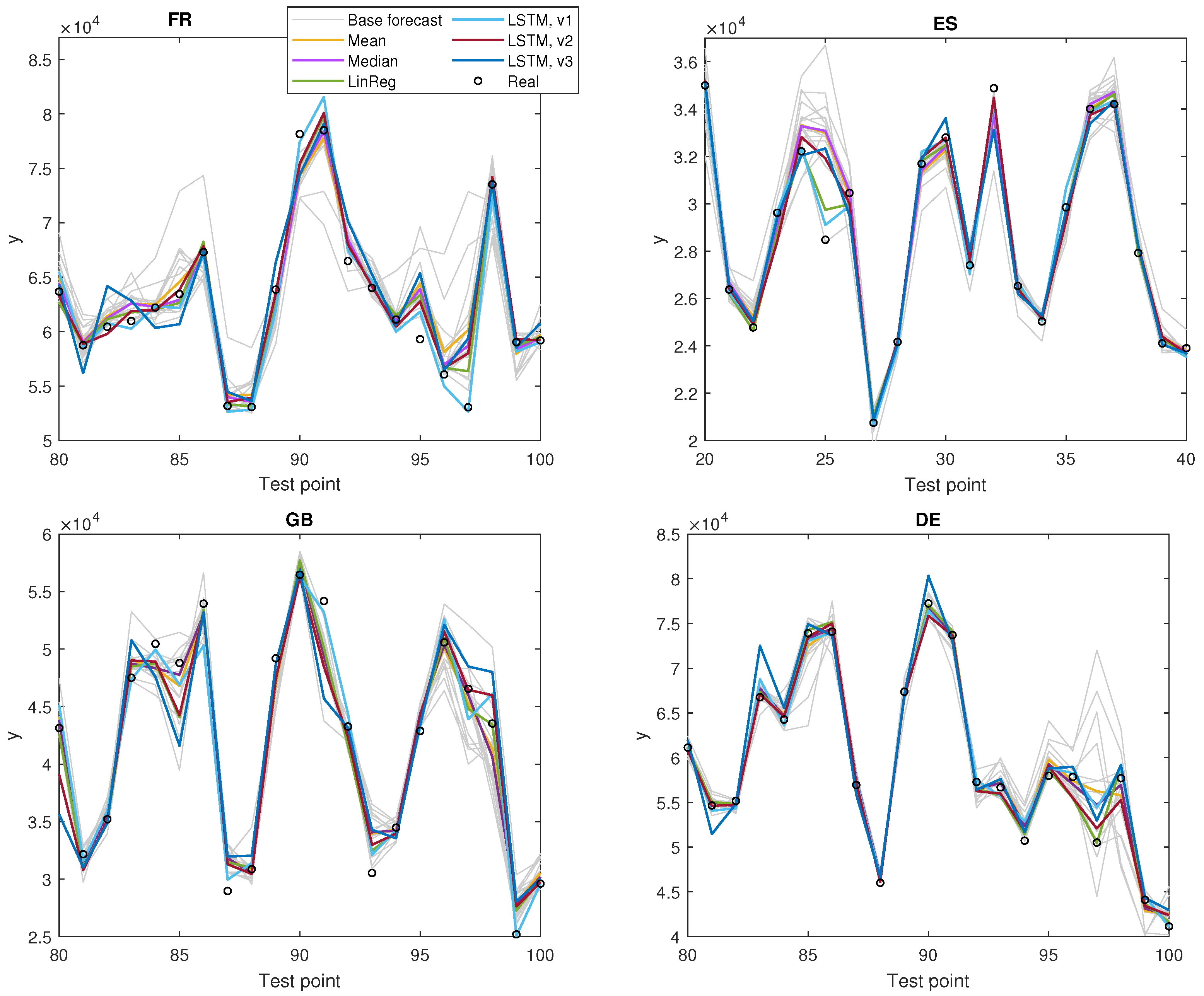
3.3. Results and Discussion

Table 1. Forecasting quality metrics for the base models.

	MAPE	MdAPE	MSE	MPE	StdPE
ARIMA	2.86	1.82	777,012	0.0556	4.60
ETS	2.83	1.79	710,773	0.1639	4.64
Prophet	3.83	2.53	1,641,288	−0.5195	6.24
N-WE	2.12	1.34	357,253	0.0048	3.47
GRNN	2.10	1.36	372,446	0.0098	3.42
MLP	2.55	1.66	488,826	0.2390	3.93
SVM	2.16	1.33	356,393	0.0293	3.55
LSTM	2.37	1.54	477,008	0.0385	3.68
ANFIS	3.08	1.65	801,710	−0.0575	5.59
MTGNN	2.54	1.71	434,405	0.0952	3.87
DeepAR	2.93	2.00	891,663	−0.3321	4.62
WaveNet	2.47	1.69	523,273	−0.8804	3.77
N-BEATS	2.14	1.34	430,732	−0.0060	3.57
LGBM	2.43	1.70	409,062	0.0528	3.55
XGB	2.32	1.61	376,376	0.0529	3.37
cES-adRNN	1.70	1.10	224,265	−0.1860	2.57

shows the forecasting quality metrics for the base forecasting models. Note the significant difference in results between the various models, with MAPE ranging from 1.70 for cES-adRNN to 3.83 for Prophet. The overall mean MAPE across all models was 2.53.

Table 2. Forecasting quality metrics for different ensemble approaches (best results in bold).

	Variant	MAPE	MdAPE	MSE	MPE	StdPE
Mean	-	1.91	1.23	316,943	−0.0775	3.11
Median	-	1.82	1.13	287,284	−0.0682	3.05
LinReg	-	1.63	1.11	213,428	0.0131	2.38
LSTM	v1, $k=168$	1.55	1.09	139,667	0.0247	2.26
LSTM	v2, global	1.95	1.34	270,266	−0.1046	2.89
LSTM	v3, global	2.97	1.84	726,108	−0.3628	4.84

shows forecasting quality metrics for different ensemble approaches. Mean and Median are just the mean and median of 16 forecasts produced by the base models. LinReg is a linear combination of these forecasts with weights estimated on the training samples $\mathrm{\Xi }=T$. As can be seen from Table 2, the most accurate approach is variant v1 of LSTM for $k=168$. This variant, which involves meta-learning on the full sequence restricted to the last 168 points, provided the most accurate results as measured by MAPE, MdAPE, and MSE errors. Note the significant difference in errors between this variant and the second most accurate ensembling method, LinReg, which achieved about 5% in MAPE and 35% in MSE.

Note that using the simplest method of combining forecasts, Mean or Median, resulted in significantly larger errors compared to LSTM v1. Unfortunately, variants v2 and v3, which excluded seasonality from the training sequence, were found to be inaccurate and did not perform well. This suggests that excluding seasonality from the training sequence could lead to the loss of important information related to the seasonal patterns in the data, resulting in deteriorated forecasting performance.

Figure 3 displays the MAPE boxplots for LSTM in three variants with varying lengths of the training sequence k. Additionally, the boxplots for the baseline methods, namely Mean, Median, and LinReg, are shown for comparison. As shown in the figure, LSTM in variants v2 and v3 are highly sensitive to the length of the training sequence. It achieved the lowest errors when trained on all available data points. Extending the training sequence may potentially further reduce errors. In contrast, for LSTM v1, the training sequences of length 168 h (one week) provided the lowest errors.

MPE in Table 2 provides information about the forecast bias, which is the lowest for LinReg, but LSTM v1, with MPE = 0.0247, is in second place. It is worth noting that Mean and Median produce more biased forecasts. The lowest value of StdPE for LSTM v1 indicates the least dispersed predictions compared to other approaches for combining forecasts.

Figure 4 depicts examples of forecasts for selected countries and test points. It is worth noting that LSTM v1 was able to achieve forecasts close to the target values, which were outside the interval of the base models’ forecasts (let us denote this interval for the i-th test point by $Z_i$) and despite the fact that no base model even came close to these targets (see test point no. 94 for FR and 99 for GB in Figure 4). One possible explanation for this ability of LSTM is the incorporation of additional information from the immediate past through internal states $\mathbf{c}$ and $\mathbf{h}$ (see (2)). LinReg, having no internal states, cannot use such information. Mean and Median approaches cannot even go beyond the interval $Z_i$.

To test the ability of LSTM v1 and LinReg to produce forecasts outside the interval $Z_i$, we counted the number of such cases out of the 3500 forecasts produced by each model. The results are shown in column $N_1$ of

Table 3. Extrapolation properties of LSTM v1 and LinReg.

	${\mathit{N}}_1$	${\mathit{N}}_2$	${\mathit{N}}_3$
LinReg	48	13	27
LSTM v1	447	192	244

. Column $N_2$ counts how many of these $N_1$ cases concern the situation where the target value also lay outside the Z-interval, on the same side as the meta-model forecast. Column $N_3$ counts the number of cases out of $N_1$ for which the meta-model produces more accurate predictions than the Median approach. It is evident from Table 3 that LSTM generates many more forecasts outside of $Z_i$ than LinReg. This may indicate better extrapolation properties of LSTM, but on the other hand, it may also suggest an increased susceptibility to overfitting.

In summary, our research findings suggest that LSTM, as a meta-learner, exhibits sensitivity to the length of the training sequence and achieves optimal performance when trained in global mode. However, it is important to note that the overall performance also depends on the accuracy and correlation of the base forecasts. In this study, we did not delve into the analysis of interdependence between the base forecasts or select the optimal set of base models. These aspects present opportunities for further optimization and improvement in future research.

LSTM poses greater challenges compared to classical ML methods such as MLP or random forests. It involves a larger number of hyperparameters and parameters that need to be tuned, making the optimization and training process more complex. Additionally, LSTM typically requires a larger amount of data to achieve optimal performance due to its ability to capture intricate temporal dependencies. In local versions of training, where shorter training sequences are used, accurate predictions with LSTM can be challenging to obtain. This highlights the importance of having sufficient training data to effectively capture the underlying patterns and dynamics of the sequential data.

4. Conclusions

This study proposes a meta-learning approach for combining forecasts based on LSTM, which has the potential to improve accuracy, particularly in cases where there is a temporal relationship between base forecasts. The study also proposes different variants of the approach for time series with multiple seasonal patterns.

The experimental results clearly demonstrate that the LSTM meta-learner outperforms simple averaging, median, and linear regression methods in terms of forecasting accuracy. In addition, LSTM has distinct advantages over non-recurrent ML models as it is capable of leveraging its internal states to model dependencies between base forecasts for consecutive time points and capture patterns in the sequential data.

Further studies could compare LSTM with other meta-learning approaches, such as feed-forward and randomized NNs, random forests, and boosted trees to determine which approach is best suited for a given forecasting problem. Moreover, selecting a pool of base models and controlling their diversity is an interesting topic that requires further investigation.

References

1. Clements, M.; Hendry, D. Forecasting Economic Time Series; Cambridge University Press: Cambridge, UK, 1998. [Google Scholar]
2. Wang, X.; Hyndman, R.; Li, F.; Kang, Y. Forecast combinations: An over 50-year review. Int. J. Forecast. 2022; in press. [Google Scholar] [CrossRef]
3. Rossi, B. Forecasting in the presence of instabilities: How we know whether models predict well and how to improve them. J. Econ. Lit. 2021, 59, 1135–1190. [Google Scholar] [CrossRef]
4. Blanc, S.; Setzer, T. When to choose the simple average in forecast combination. J. Bus. Res. 2016, 69, 3951–3962. [Google Scholar] [CrossRef]
5. Genre, V.; Kenny, G.; Meyler, A.; Timmermann, A. Combining expert forecasts: Can anything beat the simple average? Int. J. Forecast. 2013, 29, 108–121. [Google Scholar] [CrossRef]
6. Jose, V.; Winkler, R. Simple robust averages of forecasts: Some empirical results. Int. J. Forecast. 2008, 24, 163–169. [Google Scholar] [CrossRef]
7. Pawlikowski, M.; Chorowska, A. Weighted ensemble of statistical models. Int. J. Forecast. 2020, 36, 93–97. [Google Scholar] [CrossRef]
8. Poncela, P.; Rodriguez, J.; Sanchez-Mangas, R.; Senra, E. Forecast combination through dimension reduction techniques. Int. J. Forecast. 2011, 27, 224–237. [Google Scholar] [CrossRef]
9. Kolassa, S. Combining exponential smoothing forecasts using Akaike weights. Int. J. Forecast. 2011, 27, 238–251. [Google Scholar] [CrossRef]
10. Babikir, A.; Mwambi, H. Evaluating the combined forecasts of the dynamic factor model and the artificial neural network model using linear and nonlinear combining methods. Empir. Econ. 2016, 51, 1541–1556. [Google Scholar] [CrossRef]
11. Zhao, S.; Feng, Y. For2For: Learning to forecast from forecasts. arXiv 2020, arXiv:2001.04601. [Google Scholar]
12. Gastinger, J.; Nicolas, S.; Stepić, D.; Schmidt, M.; Schülke, A. A study on ensemble learning for time series forecasting and the need for meta-learning. In Proceedings of the 2021 International Joint Conference on Neural Networks (IJCNN), Shenzhen, China, 18–22 July 2021; pp. 1–8. [Google Scholar]
13. Hochreiter, S.; Schmidhuber, J. Long short-term memory. Neural Comput. 1997, 9, 1735–1780. [Google Scholar] [CrossRef] [PubMed]
14. Hewamalage, H.; Bergmeir, C.; Bandara, K. Recurrent neural networks for time series forecasting: Current status and future directions. Int. J. Forecast. 2021, 37, 388–427. [Google Scholar] [CrossRef]
15. Smyl, S.; Dudek, G.; Pełka, P. Contextually enhanced ES-dRNN with dynamic attention for short-term load forecasting. arXiv 2022, arXiv:2212.09030. [Google Scholar]
Figure 1. LSTM model.
Engproc 39 00053 g001
Figure 2. Selection of training points for LSTM.
Engproc 39 00053 g002
Figure 3. MAPE boxplots for the various ensemble variants.
Engproc 39 00053 g003
Figure 4. Base and ensemble forecasts.
Engproc 39 00053 g004