Modelling of Leishmaniasis Infection Dynamics: A Comparative Time Series Analysis with VAR, VECM, Generalized Linear and Markov Switching Models ^†

Abstract

In this paper, we are interested in modeling the dynamics of cutaneous leishmaniasis (CL) in Errachidia province (Morocco), using epidemiologic data and the most notable climatic factors associated with leishmaniasis, namely humidity, wind speed, rainfall, and temperature. To achieve our objective, we compare the performance of three statistical models, namely the Vector Auto-Regressive (VAR) model, the Vector Error Correction model (VECM), and the Generalized Linear model (GLM), using different metrics. The modeling framework will be compared with the Markov Switching (MSM) approach.

1. Introduction

Despite new developments in disease control and advanced treatment methods, leishmaniasis is still one of the most prevalent tropical diseases in the world. The World Health Organization (WHO) defines leishmaniasis as an infectious disease caused by protozoan parasites in the genus Leishmania. The transmission of the disease occurs through the bite of a sandfly infected with Leishmania parasites. Infection may be restricted to the skin in cutaneous leishmaniasis (CL), to the mucous membranes in mucosal leishmaniasis (MCL), or spread internally in visceral leishmaniasis (VL). This disease is in fact a vector-borne disease whose transmission is highly influenced by climatic factors, whereas the nature and magnitude differ between geographical regions. Further, it is known that spatial heterogeneity influences shifting patterns of vector parasite interactions, vector–host contact, and susceptibility of the population [1].

Many recent studies and research papers [2,3,4] suggest that the incidence of leishmaniasis is influenced by climatic variables. Therefore, prediction approaches are needed to achieve a better outcome in disease forecasting. In this context, the predictions made through time series analysis are extremely important in light of recent developments. This will undoubtedly help identify trends and possible disease outbreaks, which may ultimately facilitate the smooth and timely implementation of control programs through appropriate precautionary interventions.

In this paper, we compare the performance of three statistical models, namely the Vector Auto-Regressive (VAR) model, the Vector Error Correction Model (VECM), and the Generalized Linear Model (GLM), using different metrics. These models are used to measure the impact of climate change on the epidemiology of leishmaniases in Errachidia province, Morocco.

These models were selected based on a benchmarking study that showed their usefulness in explaining the dynamics in different fields. Furthermore, the time series modeling framework will be compared with the Markov Switching approach.

2. Materials and Methods

The main contribution of this study is to model cutaneous leishmaniasis (CL) dynamics in Errachidia province (Morocco) using epidemiologic data and the most notable climatic factors associated with leishmaniosis, namely humidity, wind speed, rainfall, and temperature. To achieve our objective, we use three statistical models, namely the Vector Auto-Regressive (VAR) model, the Vector Error Correction model (VECM), and the Generalized Linear Model (GLM). The modeling framework will be compared with the Markov Switching approach.

2.1. A Brief Overview of Generalized Linear Models (GLM)

Generalized Linear Models include several types of models, such as linear regression, logistic regression, Poisson regression, and Negative Binomial Regression [5]. In these models, the response variable $Y_i$ is assumed to follow an exponential family distribution. The mean ${\mu }_i$ of the response variable is often assumed to be a nonlinear function of $x_i^T\beta$. The model is given by:

$$g\left(E\right(Y\left)\right)={\beta }_0+{\beta }_1{X}_1+{\beta }_2{X}_2+\cdots +{\beta }_n{X}_n+\epsilon ,$$

(1)

where $g\left(E\right(Y\left)\right)$ specifies the link between the mean $E\left(Y\right)$ and the linear combination of predictors $X_1,X_2,\dots ,X_n$. GLMs are generally fitted using a Newton-type method, such that an iteratively re-weighted least square (IWLS) algorithm is also referred to as a Fisher Scoring algorithm [6].

Various predictor selection methods are used to compromise the stability of a final model from several nested models. Based on the significance of the predictors and their correlation values with the outcome $Y_i$ we can reduce the number of predictors. Using forward-selection or backward-elimination variable-selection algorithms, the deviance, and the AIC criterion, we can determine the best-fitting model [7]. In order to assess the relevance of GLMs, we use the residual deviance test, defined as:

$$D=2\left\{l\left(saturated\right)-l\left(\mathrm{M}\right)\right\},$$

(2)

where $l\left(\mathrm{M}\right)$ is the log-likelihood of the model M, and $l\left(saturated\right)$ is the log-likelihood of a saturated model. A saturated model is where the number of parameters is equal to the number of data points. Thus, models with high likelihoods will have low deviances, and vice versa. If the model M is correct and has $p+1$ parameters, including the intercept, then the deviance will generally approach a chi-square distribution with degrees of freedom equal to $n-(p+1)$.

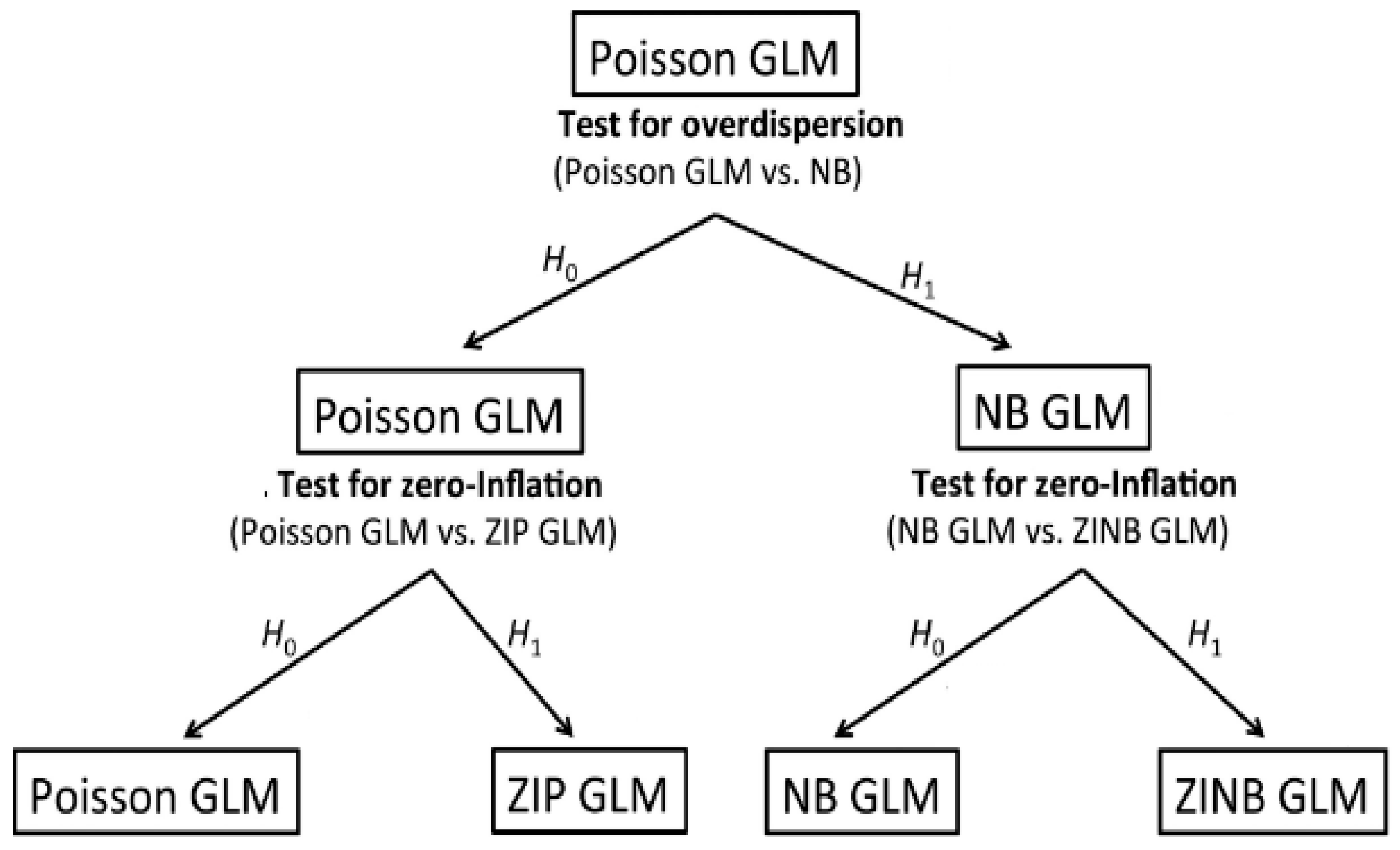
Poisson and negative binomial regression models (Figure 1) are part of the family of Generalized Linear Models that are commonly used in epidemiological studies [8]. These models are widely used to model disease incidence data with a non-negative integer, no upper limit, and highly skewed distribution. Otherwise, a zero-inflated Poisson (ZIP) model, a zero-inflated negative binomial (ZINB), or a negative binomial need to be used [9].

2.2. A Brief Overview of Multivariate Time Series Models

The Multivariate Time Series approach (Figure 2) is used to model and explain the interactions among a group of time series. In this framework, the strength of associations among different variables is expressed across time lags.

The Vector Auto-Regressive (VAR) model is one of the most commonly used techniques. It is considered as an extension of the auto-regressive model. The VAR model involves multiple independent variables and therefore has more than one equation, explaining the behavior of the relationship between endogenous variables as well as between endogenous and exogenous variables. Each equation uses as its explanatory variables the lags of all the variables and likely a deterministic trend.

If all of the original variables have unit roots and are not cointegrated, then they should be differenced and the resulting stationary variables should be used in the VAR. Let $x\left(t\right)={\left(x_1\right(t),\dots ,x_m(t\left)\right)}^{\prime }$ be an $m$-dimensional stationary process admitting the following $VAR\left(p\right)$ representation:

$$x\left(t\right)=A_1{x}_{t-1}+\cdots +A_p{x}_{t-p}+{\epsilon }_t, \mathrm{t}\in \mathbb{Z}$$

(3)

where $A_1,\cdots ,A_p$ are ($m\times m$) coefficient matrices, $p$ is the model order, and ${\epsilon }_t=\left({\epsilon }_{1t},\cdots ,{\epsilon }_{mt}\right)$′ is a ($m\times 1$) vector of white noises with $E\left[{\epsilon }_t{\epsilon }_s^{\prime }\right]=0$ for $t\ne s$ and ${\epsilon }_t\sim N(0,{\sum }_{\epsilon }).$ The coefficient matrices $A_1,\cdots ,A_p$ describe the temporal relationships within the $m$ time series in the system.

If the cointegration exists then a vector error correction model (VECM), which combines levels and differences, can be estimated instead of a VAR in levels. The VECM regression equation is given by:

$${\mathsf{\Delta }y}_t={\alpha }_1+{\rho }_1{e}_1+{\sum }_{i=0}^n{{\beta }_i\mathsf{\Delta }y}_{t-i}+{\sum }_{i=0}^n{{\delta }_i\mathsf{\Delta }x}_{t-i}+{\sum }_{i=0}^n{{\gamma }_i\mathsf{\Delta }z}_{t-i}$$

(4)

$${\mathsf{\Delta }x}_t={\alpha }_2+{\rho }_2{e}_2+{\sum }_{i=0}^n{{\beta }_i\mathsf{\Delta }y}_{t-i}+{\sum }_{i=0}^n{{\delta }_i\mathsf{\Delta }x}_{t-i}+{\sum }_{i=0}^n{{\gamma }_i\mathsf{\Delta }z}_{t-i}$$

(5)

2.3. A Brief Overview of the Markov Switching Model (MSM)

Although ARMA models are quite successful in numerous applications, they are unable to represent many nonlinear dynamic patterns such as asymmetry, amplitude dependence, and volatility clustering [10]. In addition, nonlinear time series models are not a panacea and have their own limitations. First, the nonlinear optimization algorithms easily get stuck at a local optimum in the parameter space. Second, most nonlinear models are designed to describe certain nonlinear patterns of data and hence may not be so flexible.

The Markov Switching model of Hamilton [11], also known as the regime-switching model, is one of the most popular nonlinear time series. This model involves multiple equations that can characterize the time series behavior in different regimes. By permitting switching between these structures, this model is able to capture more complex dynamic patterns. 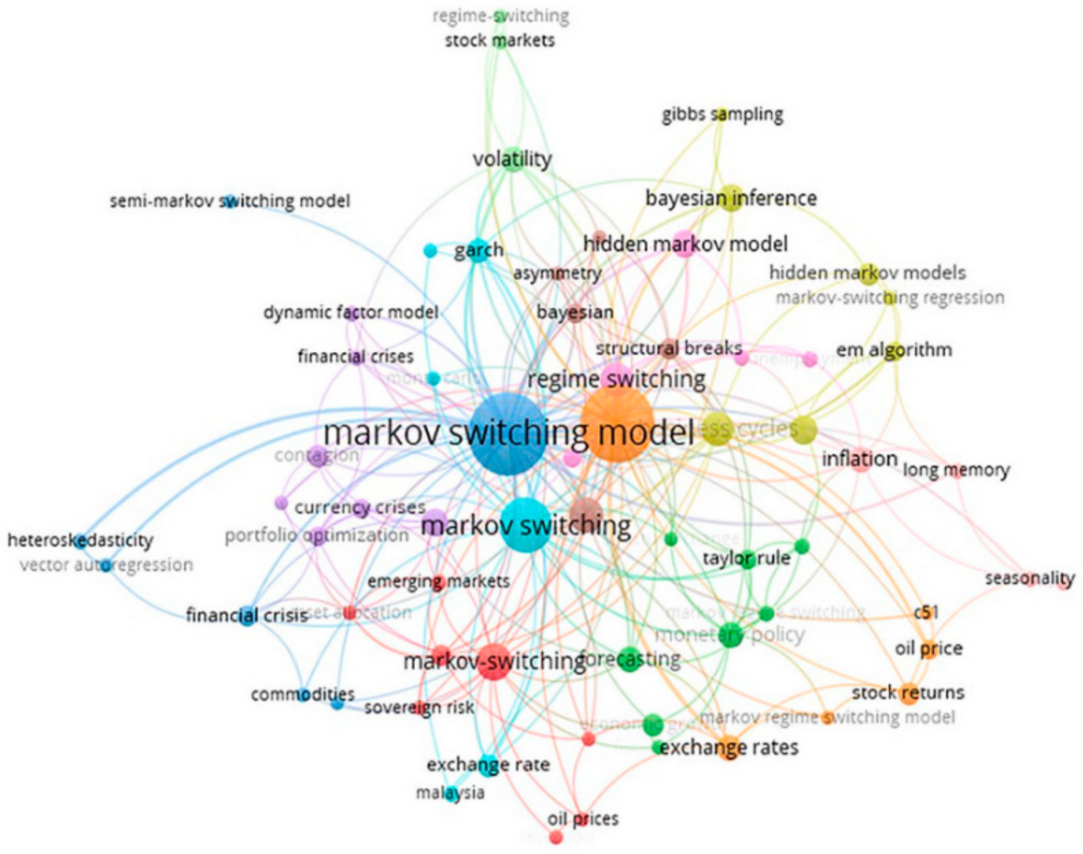This model and its variants have been widely applied [12,13]. The following network mapping [14] summarized the co-occurrence of author’s keywords when using the Markov Switching model (Figure 3).

In this network mapping, the sizes reflect the frequency of the author’s keywords in the Markov Switching literature, while the colors represent the number of clusters.

Let $s_t$ denote an unobservable state variable assuming the value of one or zero. As mentioned by Kuan (2002), a simple switching model for the variable $z_t$ involves two AR specifications:

$$z_t=\left\{\begin{array}{c}{\alpha }_0+{\beta z}_{t-1}+{\epsilon }_t, { s}_t=0\\ {\alpha }_0+{\alpha }_1+{\beta z}_{t-1}+{\epsilon }_t{, s}_t=1\end{array}\right.$$

(6)

where $\left|\beta \right|<1$ and ${\epsilon }_t$ are i.i.d random variables with mean zero and variance ${\sigma }_{\epsilon }^2$. This is a stationary AR(1) process with mean ${\alpha }_0/\left(1-\beta \right)$ when $s_t=0$, and it switches to another stationary AR(1) process with mean $\left({\alpha }_0+{\alpha }_1\right)/\left(1-\beta \right)$ when $s_t$ changes from 0 to 1. This model admits two dynamic structures at different levels, depending on the value of the state variable $s_t$. In this case, $z_t$ are governed by two distributions with distinct means, and $s_t$ determines the switching between these two distributions (regimes).

To implement our methodology and test all aforementioned modeling approaches, in this research we used monthly CL incidence data from Errachidia province and climatic variables. Data covers the period from January 2010 to December 2019.

Errachidia province is located in the Ziz Ghris Valley in the south-east of Morocco (Figure 4), including the Saharan areas, plains, and highlands at an altitude above 1900 m and covering a surface of 46,000 km². Errachidia has an arid climate with temperatures between −4 °C and 48 °C, with large daily and seasonal temperature variations. The annual mean temperature is 21 °C. Rainfall is scarce and usually occurs between February and March. The annual total precipitation is 134.64 mm [15].

3. Results and Discussions

The analysis of collected data shows that Errachidia province recorded 8487 cases of cutaneous leishmaniasis between 2010 and 2019 (Figure 5). It can be observed from Figure 5 that the monthly CL incidence peaked between 2010 and 2011, declined between 2011 and 2016, and rose around the end of 2016 to 2018. In addition, the number of CL cases had seasonal fluctuations. Most cases were recorded in the months of November, December, and January. The trend starts to increase in October, with high peaks in December and January, and declines until February. A steady-state period is observed until September.

To study the impact of climate change on the CL incidence in this region, we selected seven predictors, namely the monthly average humidity (Hmoy), precipitation (Prec), average wind speed (Vmoy), minimum temperature (Tmin), mean temperature (Tmoy), and maximum temperature (Tmax), as well as evaporation (Evap).

A linear correlation between the covariables was assessed using the Pearson coefficient, and predictors that present a strong correlation with CL cases were retained. The Spearman coefficient and the cross-correlation between the CL cases and climatic data were estimated to determine the predictors and the adequate lags to be included in the model.

Our first fitted model is Poisson regression. However, the dispersion coefficient showed severe over-dispersion (Φ_Poisson = 145.18). Thus, negative binomial regression was used as an alternative approach to model over-dispersion in the data.

The use of the stepwise method for 3- and 6-month gaps between CL cases and predictors leads to the retention of the model given by (

Table 1. Results of the stepwise selection algorithm for the 3- and 6-month gaps between CL and predictors.

GLM: Negative Binomial Models	AIC
Log(E(CL))~9.0747 Hmoy − 28.3713 Prec + 1.0572	1030.9
Log(E(CL))~6.90924 Hmoy3 + 0.18451 Tmoy3 − 2.26628	980.74
Log(E(CL))~1.20795886 Vmoy6 + 0.07317 Tmin6 − 2.34280875	932.59

Note: The bold means that this is the optimal value.

):

$$\mathrm{C}\mathrm{L}~{\mathrm{V}\mathrm{m}\mathrm{o}\mathrm{y}}_6+{\mathrm{T}\mathrm{m}\mathrm{i}\mathrm{n}}_6$$

(7)

To examine the adequacy of the fitted model, a residual diagnosis as well as the deviance test were performed.

The multivariate time-series analysis shows that data can be considered as stationary time series. The optimal VAR model identified is given by:

$$\left\{\begin{array}{c}{\mathrm{CL}}_t=0.629 {\mathrm{CL}}_{t-1}+3.326 {\mathrm{Tmoy}}_{t-1}-45.573\\ {\mathrm{Tmoy}}_t=-0.010 {\mathrm{CL}}_{t-1}+0.894 {\mathrm{Tmoy}}_{t-1}+2.844\end{array}\right.$$

(8)

To assess the performance of this model a post analysis is required. The test of the presence of serial correlation in the residual, the Portmanteau Test, shows a p-value equal to 0.0874 > 0.05, meaning that we can accept the null hypothesis of nonexistence of serial correlations.

Concerning the test of heteroskedasticity, the p-value of the arch test is equal to 0.009107 < 0.05, meaning that we reject the null hypothesis and thus the absence of heteroskedasticity.

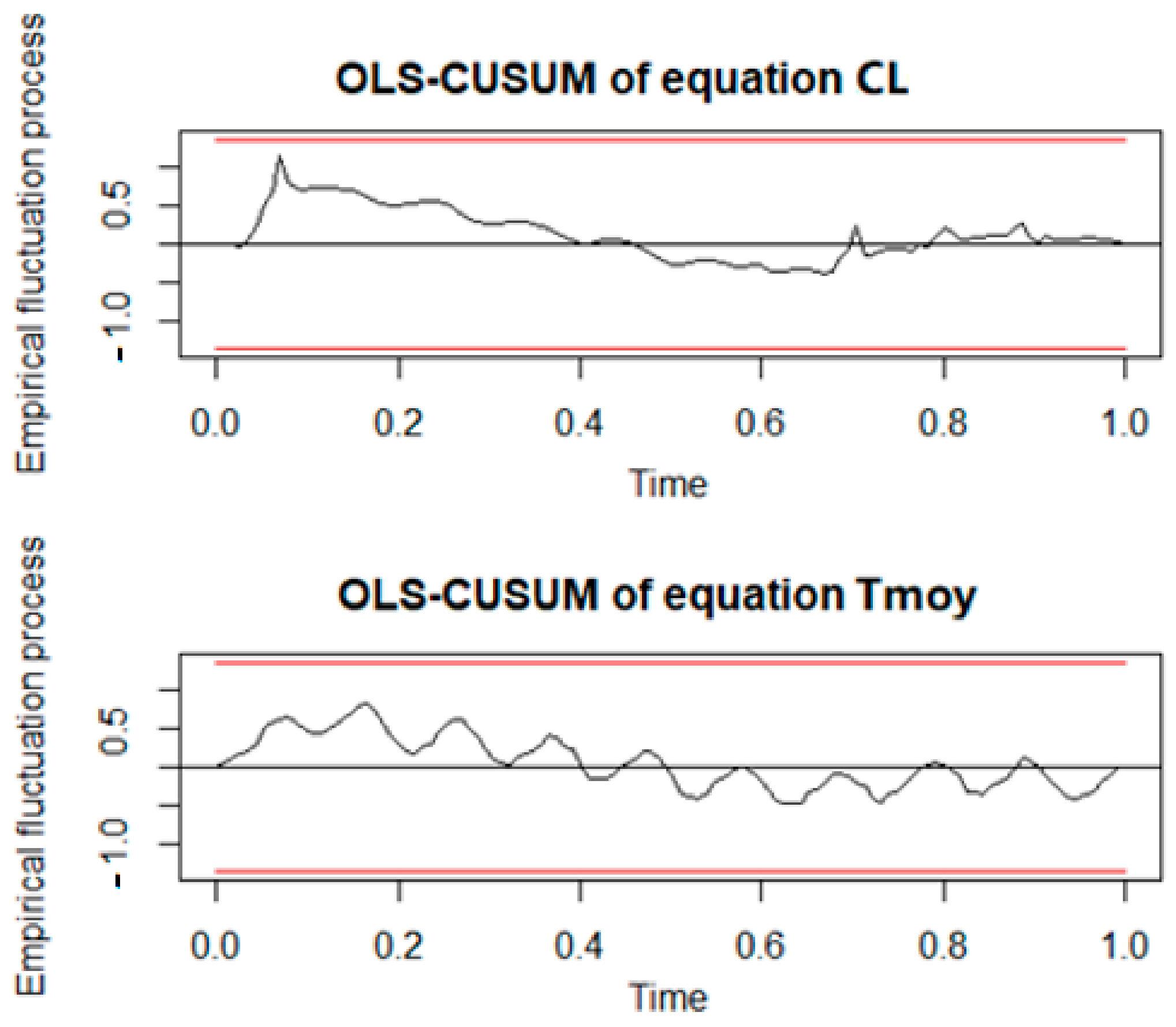
The Jarque-Bera test was then used to check if the residuals fit the normal distribution. Because the p-value is higher than 0.05, the normal distribution is accepted. The following figure (Figure 6) shows no structural break.

One of the most useful tools to characterize the dependence among time series when running the VAR model is the causality test. In our case, the objective of this test is to check if the variable “Tmoy” contributes to forecasting the “CL incidence” variable.

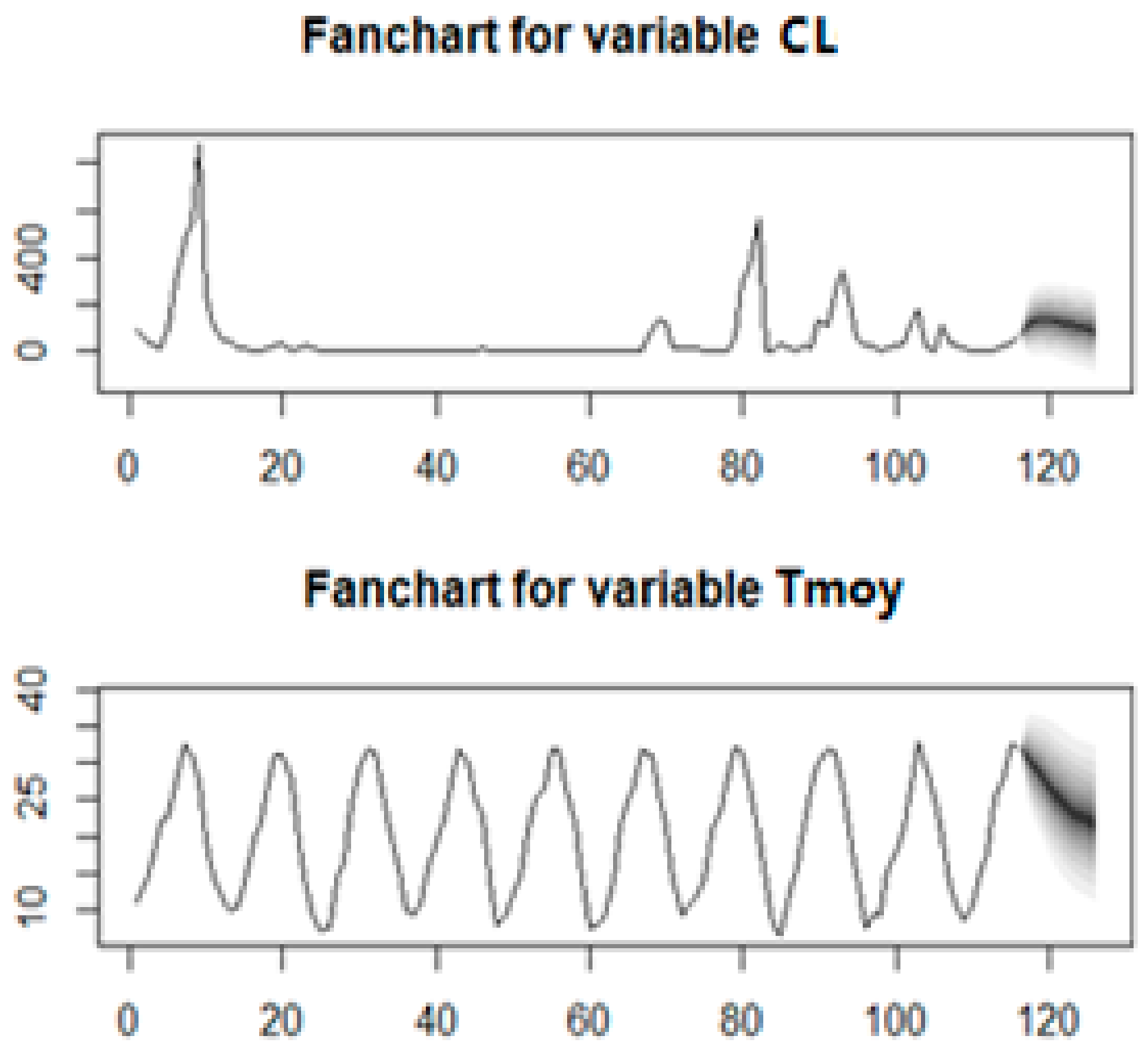
The p-value of the Granger causality test is equal to 0.0023 < 5%, meaning that we can reject the null hypothesis. Hence, “Tmoy” is considered a pertinent feature (risk factor) when predicting the “CL” variable. As displayed in Figure 7, a good performance is shown, in terms of predictions obtained from VAR(1).

The following figure (Figure 8) provides results about the Markov Switching model fitting with the estimation of regime 1 and regime 2. However, based on the AIC and residuals diagnosis, the VAR(1) performs better than the Markov Switching model.

4. Conclusions

In this study, we are interested in modeling the spread of cutaneous leishmaniasis (CL) using the Vector Auto-Regressive (VAR) model, the Vector Error Correction model, (VECM) and the Markov Switching approach (MSM). Based on our findings, we can mention that the CL time series are characterized by extreme values; therefore, it was cumbersome to explain them using meteorological data. It is worth noting that among all candidate models, the VAR model performs well in terms of underlying hypotheses such as the stationary series, so there is no need to use the VECM. In addition, the VAR model provides good results in terms of prediction. In our case, the implication of the adequacy of the VAR is that the CL variable can be considered as a function of its own past values.

It is worth noting that the VAR model is one of the most successful, flexible, and easy to use models for the analysis of multivariate time series. This model often provides superior forecasts to those from univariate time series models. In addition to data description and the underlying theory based on simultaneous equations and forecasting, the VAR is also used for structural inference.

References

- Wijerathna, T.; Gunathilaka, N.; Gunawardena, K.; Rodrigo, W. Population dynamics of phlebotomine sand flies (diptera: Psychodidae) in cutaneous leishmaniasis endemic areas of Kurunegala district, Sri Lanka. Acta Trop. 2022, 230, 106406. [Google Scholar] [CrossRef] [PubMed]
- Medenica, S.; Miladinović-Tasić, N.; Stojanović, N.M.; Lakićević, N.; Rakočević, B. Climate Variables Related to the Incidence of Human Leishmaniosis in Montenegro in Southeastern Europe during Seven Decades (1945–2014). Int. J. Environ. Res. Public Health 2023, 20, 1656. [Google Scholar] [CrossRef] [PubMed]
- Vieira, T.M.; de Oliveira Silva, S.; Lima, L.; Sabino-Santos, G.; Duarte, E.R.; Lima, S.M.; Pereira, A.A.S.; Ferreira, F.C.; de Araújo, W.S.; Teixeira, M.M.G.; et al. Leishmania diversity in bats from an endemic area for visceral and cutaneous leishmaniasis in Southeastern Brazil. Acta Trop. 2022, 228, 106327. [Google Scholar] [CrossRef] [PubMed]
- Hakkour, M.; Hmamouch, A.; Mahmoud El Alem, M.; Bouyahya, A.; Balahbib, A.; El Khazraji, A.; Fellah, H.; Sadak, A.; Sebti, F. Risk factors associated with leishmaniasis in the most affected provinces by leishmania infantum in Morocco. Interdiscip. Perspect. Infect. Dis. 2020, 2020, 6948650. [Google Scholar] [CrossRef] [PubMed]
- McCullagh, P.; Nelder, J.A. Generalized Linear Models; Monographs on Statistics and Applied Probability; Chapman & Hall: London, UK, 1989; Volume 37. [Google Scholar]
- Heinze, G.; Wallisch, C.; Dunkler, D. Variable selection—A review and recommendations for the practicing statistician. Biom. J. 2018, 60, 431–449. [Google Scholar] [CrossRef] [PubMed]
- Kianifard, F.; Gallo, P.P. Poisson regression analysis in clinical research. J. Biopharm. Stat. 1995, 5, 115–129. [Google Scholar] [CrossRef] [PubMed]
- Fekedulegn, D.; Andrew, M.; Violanti, J.; Hartley, T.; Charles, L.; Burchfiel, C. Comparison of statistical approaches to evaluate factors associated with metabolic syndrome. J. Clin. Hypertens. 2010, 12, 365–373. [Google Scholar] [CrossRef] [PubMed]
- Kuan, C.-M. The Markov Switching Model; Institute of Economics Academia Sinica: Taipei, Taiwan, 2002; Available online: http://homepage.ntu.edu.tw/~ckuan/pdf/Lec-Markov_note.pdf (accessed on 1 February 2023).
- Hamilton, J.D. A new approach to the economic analysis of nonstationary time series and the business cycle. Econom. J. Econom. Soc. 1989, 57, 357–384. [Google Scholar] [CrossRef]
- Lu, H.M.; Zeng, D.; Chen, H. Prospective infectious disease outbreak detection using Markov switching models. IEEE Trans. Knowl. Data Eng. 2009, 22, 565–577. [Google Scholar] [CrossRef]
- Van Os, B.; van Dijk, D. Accelerating peak dating in a dynamic factor Markov-switching model. Int. J. Forecast. 2023; in press. [Google Scholar]
- Bouteska, A.; Sharif, T.; Abedin, M.Z. COVID-19 and stock returns: Evidence from the Markov switching dependence approach. Res. Int. Bus. Financ. 2023, 64, 101882. [Google Scholar] [CrossRef] [PubMed]
- Phoong, S.W.; Phoong, S.Y.; Khek, S.L. Systematic literature review with bibliometric analysis on Markov switching model: Methods and applications. SAGE Open 2022, 12, 21582440221093062. [Google Scholar] [CrossRef]
- Bounoua, L.; Kahime, K.; Houti, L.; Blakey, T.; Ebi, K.L.; Zhang, P.; Imhoff, M.L.; Thome, K.J.; Dudek, C.; Sahabi, S.A.; et al. Linking climate to incidence of zoonotic cutaneous leishmaniasis (L. major) in pre-Saharan North Africa. Int. J. Environ. Res. Public Health 2013, 10, 3172–3191. [Google Scholar] [CrossRef] [PubMed]