Proceeding Paper

Forecasting Agricultural Area Using Nerlovian Model in Côte d’Ivoire †

1
Laboratoire des Sciences et Technologies de l’Environnement (LSTE), Université Jean Lorougnon GUEDE, Daloa P.O. Box 150, Côte d’Ivoire
2
Laboratoire de Recherche en Economie et Gestion (LAREG), Université Jean Lorougnon GUEDE, Daloa P.O. Box 150, Côte d’Ivoire
*
Author to whom correspondence should be addressed.
Presented at the 9th International Conference on Time Series and Forecasting, Gran Canaria, Spain, 12–14 July 2023.
Eng. Proc. 2023, 39(1), 35; https://doi.org/10.3390/engproc2023039035
Published: 29 June 2023
(This article belongs to the Proceedings of The 9th International Conference on Time Series and Forecasting)

Abstract

:
In this article, we develop the Nerlove models that give the area of cacao and cashew nuts in terms of the area, the price and the rainfall. These models are estimated using the methods of ordinary least square and likelihood maximum and are used to analyze the link in a short time between the agricultural determinants. The results showed that the anticipation elasticity had an effect on the price practiced and forecast model. In a short time, the price delayed by one year, and the area delayed by one and two years, had decreasing returns to scale for the current area.

1. Introduction

The agricultural sector has always been one of the pillars in the Ivorian economy. As the world’s leading producer of cocoa beans and the cashew nuts, Côte d’Ivoire is a key country in this sector. Export agriculture (coffee and cocoa) has long been the mainstay of the economy. Despite the emergence of a growing industrial fabric and the government’s commitment to invest in other sectors such as education, Ivorian agriculture continues to contribute significantly to government revenues. Thus, in 2021, the agricultural sector represented 20% of Côte d’Ivoire’s GDP and 60% of the country’s exports in 2018. The agricultural sector employs 46% of the workforce and provides a living for two-thirds of the population.
After independence, Côte d’Ivoire inherited cocoa. Its production, which was 1.5 million tons in 1964, reached the mark of 4.162 million tons in 2013–2014 [1]. It has now become one of the most profitable crops in the world, generating 7.4 billion USD in 2008 among small producers [2]. In contrast, cashew nuts were introduced in northern Côte d’Ivoire in the late 1950s for reforestation and soil protection. Progressively, from a purely ecological aspect, the establishment of the cashew tree met a socio-economic need, since this tree can produce marketable nuts. Thus, cashew became a real speculation from the 1990s, due to the increasing demand for cashew nuts on the international market. The cashew sector has thus experienced spectacular development, with national production of raw cashew nuts increasing from 19,000 tons in 1990 to about 750,000 tons in 2018.
In Cote d’Ivoire, the development of the agricultural sector has had a significant and considerable impact on the economic and social well-being of the population. The economy of Côte d’Ivoire is still based on the exploitation and export of raw materials, mainly agricultural materials [3]. This economy is much more oriented towards the analysis of agricultural supply. This consists of analyzing the supply response to product prices and to the prices of production factors and intermediate consumption. This analysis also concerns the agricultural income of suppliers (producers). Producers are rational economic agents who offer the total quantity of a good on the market in exchange for a price.
Several econometric models have based their studies on the relationship between agricultural determinants such as supply and price. We can cite the work of Nerlove, who was the first to develop a theory known as “the Nerlovian models of supply response” in 1956 and 1958. This article is part of the econometric modeling and forecasting of agricultural determinants based on the Nerlove model. The first part aims at estimating the price elasticities of the agricultural products cocoa and cashew nuts and analyzing their effects on forecasting using the Nerlove model. In the second part, we develop an estimation technique for the parameters of the Nerlove model, based on the maximum likelihood method. This study is applied to data on rainfall, agricultural areas and prices paid to farmers in Côte d’Ivoire over the period 1980–2022.

2. Materials and Methods

According to Nerlove [4,5] the most robust starting point to determine what is likely is to assume that the expectation price of agricultural determinants depend on past price values. Nerlove defined the adjustment coefficient as a ratio between the actual price variation and the expected price change. This assumption is similar to that of Cagan’s [6] theory of adaptive expectations, which states that “The expected rate of price change is revised in each period in proportion to the deviation of the observed rate of price change from the previously expected rate of price change”.

2.1. Specification of the Nerlove Model of the Cultivated Area

The basic Nerlove model formed by the three hypotheses is, thus, finally written
S F t e = a 0 + a 1 P t a + a 2 Z t + u t P t a = P t 1 a + β P t 1 P t 1 a S F t = S F t 1 + δ S F t e S F t 1
where S F t e is the area desired; S F t is the area practiced; P t a is the expected price deemed “normal” by producers in period t; P t is the actual price in period t; β is the “expectation coefficient”, or “anticipation elasticity”, it is the correction factor assumed constant and such that 0 β 1 ; and a 0 , a 1 , a 3 and δ are adjustment coefficients.
Nerlove said that the actual change in area is a proportion of the difference between the equilibrium level of area (noted δ ) and the area actually cultivated in the previous period. Eliminating the unobservable variable S F t e using the Koyck transformation [7], we consider that the random variable u t is a white Gaussian noise if V t is a moving average process of order 1 (MA(1) or ARMA(0, 1)).
Model (1) can still be written as follows:
S F t 1 β 2 S F t 2 = b 1 + b 2 P t 1 + b 3 S F t 1 1 β S F t 2 + b 5 Z t 1 β Z t 1 + V t

2.2. Estimation of the Cultivated Area Model

We estimated the parameter β from the second equation of Model (1) with the method of ordinary least squares (OLS). The estimated parameter was denoted β ^ .
The β ^ statistic was injected into Model (2) and we also estimated the other parameters with the OLS method.
The estimation errors of the OLS method, denoted V t , must be independent and identically distributed (normal distribution). In some cases, we had assumptions that were not verified; then, the models were adjusted with the maximum likelihood method. In this case, the estimation errors must be a moving average process of order 1.
(a) 
Estimation of the β parameter
From Equation (1), we derive the following linear fitting model:
P t a = P t 1 a + β P t 1 P t 1 a + u t ,
where u t is the assumed independent and identically distributed normal distribution error term. Using the OLS method, we obtained the expression for the estimator β ^ of the parameter β defined by
β ^ = t = 1 T P t 1 P t 1 a P t a P t 1 a t = 1 T P t 1 P t 1 a 2
(b) 
Ordinary least squares method (OLS)
In Model (2), we denote
λ = 1 β ^   and   y t = S F t λ 2 S F t 2
Then, the model is written
y t = b 1 + b 2 P t 1 + b 3 S F t 1 λ S F t 2 + b 5 Z t λ Z t 1 + V t .
In matrix form, the multiple regression model is written (the matrix for Model (3)) is
Y = X B + V ,
with
Y = y 1 y 2 y 3 y 4 y T ,   X = 1 P 0 S F 1 λ 2 S F 1 Z 1 λ Z 0 1 P 1 S F 1 λ S F 0 Z 2 λ Z 1 1 P 2 S F 2 λ S F 1 Z 3 λ Z 2 1 P 3 S F 3 λ S F 2 Z 4 λ Z 3 1 P T 1 S F T 1 λ S F T 2 Z T λ Z T 1
B = b 1 b 2 b 3 b 5   and   V = V 1 V 2 V 3 V 4 V T .
We obtained the estimator B ^ of B defined by
B ^ = b ^ 1 b ^ 2 b ^ 3 b ^ 5 = X X 1 X Y .
(c) 
Maximum likelihood method
For this method, we used Model (2) with the error term V t = δ u t 1 β u t 1 , which is a moving average of order. Model (2) is written
y t = b 1 + b 2 P t 1 + b 3 S F t 1 λ S F t 2 + b 5 Z t λ Z t 1 + δ u t λ u t 1
The model is then rewritten
Y = X B + A U ,
with
A = δ 0 0 0 0 λ δ δ 0 0 0 0 0 0 λ δ 0 0 δ λ δ 0 0 δ 0 0 δ λ δ 0 0 δ   and   U = u 1 u 2 u 3 u 4 u T 1 u T .
We have
Y = X B + A U A U = Y X B U = A 1 Y X B
The vector U is a vector whose components are Gaussian noise. Therefore,
U = A 1 Y X B ~ N 0 0 0 0 ; σ ² I T
where I T is the identity matrix of order T.
The density function of the vector U is given by
f u 1 , , u T = 1 2 π T / 2 1 σ ² T / 2 e x p 1 2 A 1 Y X B 1 Y X B ,
where = σ ² I t and 1 = 1 σ ² I t .
The likelihood can be written as follows
L b 1 , b 2 , b 3 , b 5 , σ = t = 1 T 1 2 π 1 / 2 1 σ ² 1 / 2 e x p 1 2 σ ² A 1 Y X B A 1 Y X B .
We show by recurrence that:
A 1 = 1 δ λ 0 0 0 0 0 λ 1 λ 0 0 0 0 λ 2 λ 1 λ 0 0 0 λ 3 λ 2 λ 1 λ 0 0 λ 0 λ T 1 λ T 2 λ T 3 λ 1 λ 0
We can easily define the likelihood
L b 1 , b 2 , b 3 , b 5 , σ = 1 2 π T / 2 1 σ ² T / 2 e x p 1 2 σ 2 δ 2 t = 1 T j = 1 t λ t j y t j + 1 k = 1 4 X t j + 1 ; k B k 2
The log-likelihood is given by
l o g L b 1 , b 2 , b 3 , b 5 , σ = T 2 l o g 2 π σ 2 1 2 σ 2 δ 2 t = 1 T j = 1 t λ t j y t j + 1 k = 1 4 X t j + 1 ; k B k 2 .
We obtained the optimal values of the parameters by maximizing the log-likelihood function. To do this, we have
l o g L b 1 , b 2 , b 3 , b 5 , σ = 0 .
We used the first four equations. We obtained
S t = 1 T j = 1 t X j ; 1 λ t j y j X j ; 1 b 1 X j ; 2 b 2 X j ; 3 b 3 X j ; 4 b 5 = 0 t = 1 T j = 1 t X j ; 2 λ t j y j X j ; 1 b 1 X j ; 2 b 2 X j ; 3 b 3 X j ; 4 b 5 = 0 t = 1 T j = 1 t X j ; 3 λ t j y j X j ; 1 b 1 X j ; 2 b 2 X j ; 3 b 3 X j ; 4 b 5 = 0 t = 1 T j = 1 t X j ; 4 λ t j y j X j ; 1 b 1 X j ; 2 b 2 X j ; 3 b 3 X j ; 4 b 5 = 0 .
We developed each equation of the system (S) and applied the double sum on each term to write our system (S) in matrix form. We obtained the following matrix equation
N = M B B = M 1 N
where M is a symmetric matrix given by
M = M 11 M 21 M 31 M 12 M 13 M 14 M 22 M 23 M 24 M 32 M 33 M 34 M 41 M 42 M 43 M 44   N = t = 1 T j = 1 t X j ; 1 λ t j y j t = 1 T j = 1 t X j ; 2 λ t j y j t = 1 T j = 1 t X j ; 3 λ t j y j t = 1 T j = 1 t X j ; 4 λ t j y j   and   B = b 1 b 2 b 3 b 5 .
We denoted
t j + 1 = j , M i k = t = 1 T j = 1 t X j   ; i X j   ; k λ t j   and   i , k ϵ 1,2 , 3,4 .
We define Equation (5) from the gradient of the log-likelihood function given by Equation (4).
1 σ 3 δ 2 t = 1 T j = 1 t λ t j y j X j ; 1 b 1 X j ; 2 b 2 X j ; 3 b 3 X j ; 4 b 5 2 = T
After the computation the estimator B ^ of the parameter matrix B, we injected the estimated values b ^ 1 , b ^ 2 , b ^ 3   a n d   b ^ 5 into Equation (5) of our system (S) to calculate the estimated variance σ ^ 2 of the errors.

2.3. Data

This study was carried out on two types of agricultural products most practiced in Côte d’Ivoire. It was, in particular, about cocoa and cashew nuts, where Cote d’Ivoire occupies the first world rank. These two agricultural products were chosen because they contribute significantly to reducing poverty in Côte d’Ivoire. The determinants of cocoa and cashew used in our study were the cultivated area (hectare), the effective price (field price), the average annual rainfall in the Savane and Denguélé regions where the cashews are produced and the average annual rainfall (in millimeters) in the southeast, east, central-east, central-west, central and west, where cocoa is produced. The cultivated area was assumed to be the harvested area that is relatively available. The effective price was the edge-of-field price, which is the price at which a kilogram of cocoa or cashew nuts is purchased from the producer (farmer). Our data for cashew nuts were collected from the databases of the Cotton and Cashew Council (CCA), the Food and Agriculture Organization (FAO) and SODEXAM. These data cover the period from 1990 to 2019 (sample of 30 observations). For cocoa, the data for our study came from the databases of the Coffee-Cacao Council, the World Bank and the FAO (Food and Agriculture Organization). These data cover the period from 1980 to 2020 (sample of 41 observations). We worked with 26 observations for the cashew nut variables and 38 observations for the cocoa variables. In any case, the four remaining observations were used to test the predictive quality of our models.

3. Results and Discussions

3.1. Estimation of the Elasticity Coefficient

The elasticity estimation for the cashew nuts was calculated by assuming the expected price to be within the range of prices announced by the board. We had P t a P m i n , P m a x , where [ P t , m i n , P t m a x ] is the range of prices charged to buyers of the cashew nuts given by Cotton and Cashew Council. The effective price ( P t ) was the average annual price practiced. We assumed the expected price of cocoa ( P t ) as the average annual market price. The actual price was the field price of cocoa. The results are given in the following.
The price elasticity coefficients in Table 1 are included in [0, 1].
  • For the cashew nuts: we remark that the elasticities β m i n , β q 3 and β m a x of the minimum, third quartile and maximum prices, respectively, were moderately sensitive to the prices actually practiced. On the other hand, the elasticities β q 1 and β m e d , respectively, of the first quartile and median prices were highly sensitive to the price practiced.
  • In the case of cacao, we also noted a low sensitivity of the stock market price in relation to the field price of cocoa.
These estimated values of the elasticities were then fixed in the Nerlove model to estimate the parameters of the model.

3.2. Estimation of the Nerlove Model Parameters of the Cultivated Area

Cashew nuts:
We estimated the parameters using the OLS method. These estimates were made to calculate the elasticity values because they presented the best conditions of estimation.
The results of the estimates are given in Table 2.
Table 2 presents the estimated parameters of the Nerlove model of the cultivated area of cashew nuts using OLS. The results show that the good quality given by the R 2 was close to one. The residuals of these models were independent and identically Gaussian. The estimated Models 1, 2, 3 and 4 are given by the following equation:
l o g ( S F t ) = b ^ 1 + b ^ 0 l o g ( λ 2 S F t 2 ) + b ^ 2 P t 1 + b ^ 3 log S F t 1 λ S F t 2 + b ^ 5 Z t λ Z t 1 + V t .
The last model, 5, is given by
S F t = b ^ 1 + b ^ 0 λ 2 S F t 2 + b ^ 2 * P t 1 + b ^ 3 S F t 1 λ S F t 2 + b ^ 5 Z t λ Z t 1 + V t ,
where V t ; t = 1,2 , ; n is the residual of the model, independent and normally distributed; and λ = 1 β .
Cacao:
The estimation of the Nerlove model with the cocoa data was done using the maximum likelihood method. The residuals of this model did not respect the assumptions required by the OLS method. Table 3 presents the results of the estimation using the maximum likelihood method.
The results show that all the variables, namely the delayed cocoa price, the delayed area of one and two periods, rainfall and the delayed rainfall of one period, statistically and significantly permit explanations for the variations in the area actually practiced and, therefore, in the supply of cocoa in Côte d’Ivoire. Nervole model of the cocoa did not give the good prediction qualities. For this reason, we used models 1, 2, 3 and 4 to predict the area practiced for the cashew nuts.

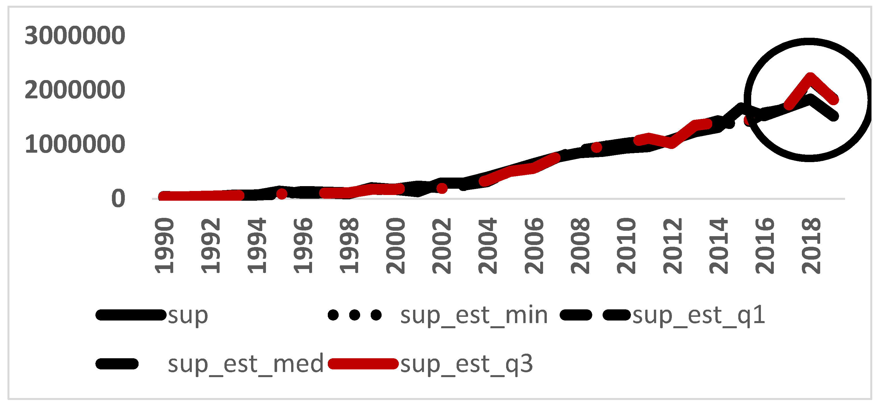
3.3. Forecast of Cashew Area

In this section, we present the prediction results of our estimated cashew model. Figure 1 shows the graphs of the cultivated area and the predictions of Models 1, 2, 3 and 4. For the choice of the best model, we compared the results of the Root of the Sum of the Mean Squares (RSMS) of the bias. We calculated the bias between the practiced area and the cultivated area estimated by the model. We define the bias by:
B i a i s t = S u r f t S u r f t , e s t i m S u r f t , e s t i m   and   R S M S = 1 N 1 t N B i a i s t 2
The results in Table 4 show that the RSMS of the practiced areas and those given by the different models are quite close. The bias was calculated with 26 observations used in our model estimation. Table 5 shows the RSMS between the four observations that were conserved and those given by the estimated models. We can see that the RSMS are also quite close.
We noticed that Models 2 and 3 gave smaller RSMS results. The expectation coefficients (anticipation elasticity) calculated from the median and first quartile expected prices contributed to the better fit of the Nerlove model of the practiced area.
The circled portion of Figure 1 shows the predictions of the estimated Models 1, 2, 3, 4.

3.4. Discussion

To apply the logarithm, the estimated parameters were considered as elasticities at short times in Models 1, 2, 3 and 4 [8]. The practiced area delayed by one year and two years had positive coefficients. This means that they contributed positively to the variation of the practiced area. On the other hand, the coefficient of the variation price ( b ^ 2 ) of the cashew nuts was not positive. This variable contributed negatively to the variation in the practiced area. The sum of the elasticities of the practiced area delayed by one year, by two years and the price variation of the cashew nuts were positive and less than one. This is decreasing returns to scale. This means that when all factors of production are increased by one unit (1%), supply will decrease by one unit (1%). These determinants of production contributed significantly and decreasingly to explain the area variation in cashew nuts.
The coefficient of the rainfall factor was not significant and positive. The effect of rainfall was negligible (short time) in the supply variation of cashew nuts. The significance of the parameters and the RSMS results (Table 5) indicated that Models 2 and 3 were better fits for the areas of the cashew nuts. They give good predictions for the practiced area. When the sum of the elasticity of cocoa was equal to one, then we had constant returns to scale. Indeed, if we increase or decrease the variables (factors of production) by 1%, then the supply will also increase or decrease by 1%. The estimated parameters represent the elasticities in a short period. The estimated value of β, which corresponded to the elasticity of anticipation, was 0.012 or 1.2%, which means that Ivorian producers assume that the price in the current period is equal the sum of 98.8% of the price anticipated in the previous period and 1.2% of the actual price.

4. Conclusions

This study considers the relationships between certain factors of production in Côte d’Ivoire. Using the Nerlove model, the econometric results of the study confirm that even in Côte d’Ivoire, the price variation has a negative effect on supply. Nerlove’s econometric model, which is a pioneering model of farmer behavior and has been used in a multitude of studies around the world, with quite variable results [9] allowed us to show in this study that price (delayed), rainfall (current and delayed) and area (delayed by one and two periods) are key variables in production decisions for farmers. Producers are positively sensitive in the short run to the variation in delayed price, area and all other supply determinants except current rainfall. Thus, over the study period, changes in price, area delayed by one and two years and rainfall delayed by one period contributed differently to increasing cocoa and cashew supplies in Côte d’Ivoire.

Author Contributions

G.C.O.: Conceptualization, methodology, software, formal analysis, visualization, investigation and writing—original draft preparation. K.K.: Conceptualization, validation, methodology, software and writing—original draft preparation. Y.A.N.: Methodology, validation and review. A.K.K.: Conceptualization, validation and review. All authors have read and agreed to the published version of the manuscript.

Funding

This research received no external funding.

Institutional Review Board Statement

Not applicable.

Informed Consent Statement

Not applicable.

Data Availability Statement

Databases of the Coffee Cacao Council (ICCO), the Cotton Cashew council in Côte d’Ivoire and SODEXAM.

Acknowledgments

The authors would like to thank the anonymous referees for their constructive comments that improved the quality of this paper.

Conflicts of Interest

The authors declare no conflict of interest.

References

  1. ICCO. Quarterly Bulletin of Cocoa Statistics; Cocoa Year 2013/2014; ICCO: London, UK, 2014. [Google Scholar]
  2. ICCO. Quarterly Bulletin of Cocoa Statistics; Cocoa Year 2017/18; ICCO: London, UK, 2008. [Google Scholar]
  3. PND 2016–2020, Groupe Consultatif, Plan National De Developpement, Côte d’Ivoire. Available online: http://www.caidp.ci/uploads/506b0bce6be504b64d5359c6407cd7df.pdf (accessed on 1 January 2016).
  4. Nerlove, M. Estimates of the Elasticities of Supply of Selected of Agricultural Commodities. J. Farm Econ. 1956, 38, 496–509. [Google Scholar]
  5. Nerlove, M. The Dynamics of Supply: Estimation of Farmers Response to Price; John Hopkins University Press: Baltimore, MD, USA, 1958. [Google Scholar]
  6. Cagan, P. The Monetary Dynamics of Hyperinflation. In Studies in the Quantity Theory of Money; Friedman, M., Ed.; University of Chicago Press: Chicago, IL, USA, 1956; pp. 25–117. [Google Scholar]
  7. Koyck, L.M. Distributed Lags and Investment Analysis; North-Holland Publishing Company: Amsterdam, The Netherlands, 1954. [Google Scholar]
  8. Gujarati, D.N. Basic Econometrics, 4th ed.; McGraw-Hill Companies: Singapore, 2004. [Google Scholar]
  9. Askari, H.; John, T. Cumming, Agricultural Supply Response: A Survey of the Econometric Evidence; Praeger Publishers: Westport, CT, USA, 1977. [Google Scholar]
Figure 1. Graph of Nerlove model predictions of cashew nut.
Engproc 39 00035 g001
Table 1. Estimation of the elasticity coefficients.
Variables Anticipation ElasticityEstimated Values
Cacao β 0.012
Cashew nuts β m i n 0.37
β q 1 0.71
β m e d 0.65
β q 3 0.31
β m a x 0.23
Table 2. Parameters estimated using the OLS method.
ModelsAnticipation Elasticity b ^ 1 b ^ 0 b ^ 2 b ^ 3 b ^ 5 R 2 p Value DW
1 β m i n 1.716 **0.694 ***−0.00114 *0.268 **−0.00270.96650.8602
2 β q 1 2.092 **0.514 ***−0.001120.459 **−0.00160.96470.8018
3 β m e d 1.992 **0.545 ***−0.00113.0.427 **−0.001730.96490.8143
4 β q 3 1.696 **0.7469 ***−0.00112 *0.209 **−0.00310.96680.8543
5 β m a x −1.752 × 10⁶ **1.708 × 10⁵ ***4.546 × 102.046 × 100 ***−1.381 × 1030.92210.01856
*** significance to 1%, ** to 5% and * to 10%, R 2 , the coefficient of determination. p value test, Durbin–Watson.
Table 3. Parameters estimated using the maximum likelihood method.
ModelElasticity b ^ 1 b ^ 2 b ^ 3 b ^ 5
6 β c a c a o 0.3750.0100.002−0.001
Table 4. RSMS results of the estimated values.
Model1234
R S M S 0.028416960.028420180.028419730.02841385
Table 5. RSMS results of the predicted values.
Model1234
R S M S 0.01094370.010709020.010728220.01119934
Disclaimer/Publisher’s Note: The statements, opinions and data contained in all publications are solely those of the individual author(s) and contributor(s) and not of MDPI and/or the editor(s). MDPI and/or the editor(s) disclaim responsibility for any injury to people or property resulting from any ideas, methods, instructions or products referred to in the content.

