Abstract
Landslides are nonstationary and nonlinear phenomena, which are often recorded as high-dimensional vector time series manifesting spatiotemporal dependence. Contemporary econometric methods use error-correction cointegration (ECC) and vector autoregression (VAR) to handle the nonstationarity but ignore the nonlinear trend. Here, we improve the ECC-VAR methodology by inserting a nonlinear trend into the model and nonparametrically estimating it by penalised maximum likelihood, and name this method ECC-VAR-. Assisted by the empirical dynamic quantiles (EDQ) dimension reduction technique, it is sufficient to apply ECC-VAR- to just a small number of representative EDQ series to surmise the whole dataset. The application of this ECC-VAR- is well fitted to the real-world slope dataset () that consists of 1803 time series, each having 5090 time states. In addition to the forecast values, we also provide three risk assessments to predict locations, time and risk of a future failure with quantified uncertainty for building an early-warning system (e.g., predicted time of failure (ToF), where the minimum error is 2.7 h before the actual ToF).
1. Introduction
Recent advancements in modern technologies such as radars, satellites, sensors make it computationally feasible and accurate in monitoring the real-world complex systems [1,2,3]. Based on these advanced detection technologies, a move from a conventional detection–diagnosis–mitigation to a more proactive prediction–prognosis–prevention paradigm is becoming increasingly evident. A typical example is the prediction of geological hazards such as landslides. It is crucial to make reliable and timely predictions of an impending hazard for risk mitigation to protect lives, livelihoods and the environment [4,5]. However, observations of landslides are often recorded as high-dimensional, spatial–temporal-dependent vector time series with nonlinear and nonstationary phenomena. Time series forecasting of such complex systems are considered one of the emerging challenges of modern science [6].
The current existing methods for modelling and forecasting time series, for example [7,8,9,10,11], have some limitations in dealing with the diverse combinations of the nonlinear and nonstationary dynamic behaviours among the system and the computational infeasibility caused by high dimensions in the real-world dataset. The objective of this paper is to develop a statistical model used for high-dimensional, spatial–temporal-dependent, nonlinear and nonstationary time series–here, we focus on landslides—and provide reliable and timely prediction for early warnings.
We develop a data-driven model by combining several advanced techniques. First, we apply a dimension reduction technique called empirical dynamic quantiles (EDQ), proposed by Peña et al. [12] to present the high-dimension vector time series by a small number of EDQ series; then, we use error-correction and cointegration (ECC) form of the vector autoregession (VAR) model to deal with the nonstationarity in the time series and combine this with an empirical function used to capture the nonlinearity. To assess the performance of the proposed ECC-VAR--EDQ model, we apply it to real-world ground motion data, which have 1803 time series, with each having 5090 time states in total. Once we obtain the optimal model, we can calculate the forecast values and use them for further analysis to predict future failure.
The performance of a forecasting framework is not just about how accurately the forecast values can figure out the failure (i.e., true positive), it is also about how well the forecasting framework can confidently forecast a stable region (i.e., true negative). The studied slope data in this paper have both failure and stable regions, which is an ideal case for assessing our model. In addition to the forecast values that can be obtained from our proposed model, we also provide three risk assessments to predict the locations of failure, time of failure and risk of failure with quantified uncertainty, based on certain what-if-scenarios at each future time and location. From the forecast values and these three assessments, our developed forecasting framework can successfully tackle the high-dimension, nonstationary and nonlinearity among the spatial–temporal-dependent dynamic system, forecast the failure and stable in the slope data domain and provide a reliable prediction for early warnings, as shown later in the paper.
This paper is organized as follows. The slope data analysed in this paper are introduced in Section 2. The details of the method are described in Section 3 before we apply this method to the slope data in Section 4. The forecast results and three risk assessment discussions used for building an early warning system are presented in Section 5, and the conclusion about this forecasting framework is presented in Section 6.
2. Data Description
The studied slope data focus on a rock slope of an open-pit mine dominated by intact igneous rock that is heavily structured or faulted by many naturally occurring discontinuities [13]. Since the mine operation, location and year of the rock slides are confidential, we call this dataset Slope X data. The monitoring domain stretched to around 200 m in length and 40 m in height. Movements of the rock face were monitored over a 3-week period: 10:07 May 31 to 23:55 June 21. Displacement at each of the 1803 monitoring locations or pixels on the surface of the rock slope was updated every six minutes, with time states in total. This led to a vector time series data with dimensions 1803 and length 5090. A landslide occurred on the western side of the slope on June 15, with an arcuate back scar and a strike length of around 120 m. The time of failure (ToF) occurred at around 13:10 June 15 (), close to when the global peak velocity of 33.61 mm/h was reached [13,14]. The observed displacement and locations are shown in Figure 1.
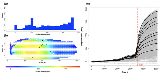
Figure 1.
(a) Displacement histogram at time of failure (ToF), 13:10 June 15. (b) Displacement at all these 1803 monitoring locations. (c) The observed 1803 time series each has length 5090 in grey. The 11 EDQ series highlight in black in (c) and their corresponding locations showed as black dots in (b). The red dashed line is the ToF.
3. Method
Limited by computational infeasible for big spatial–temporal-dependent data, most of the existing models for geo-hazards [7,8,10] can only deal with univariate or low-dimension vector time series. To improve this limitation, our proposed data-driven model forecasts future behaviors for all time series in the study domain. This model accounts for the influence of past and present at location i and all nearby locations, as well as the changes in these interdependences across space and time. The forecasts from the existing geo-hazards forecasting model often lack quantification of the associated uncertainties in terms of probabilistic assessments. The method described in this paper provides new insights in the modeling of high-dimensional, spatial–temporal-dependent time series with nonlinear and nonstationary phenomena and provides a reliable prediction of where and when failure will occur, as well as the quantified uncertainty of a future failure. An overview of our forecasting framework is presented in Figure 2.
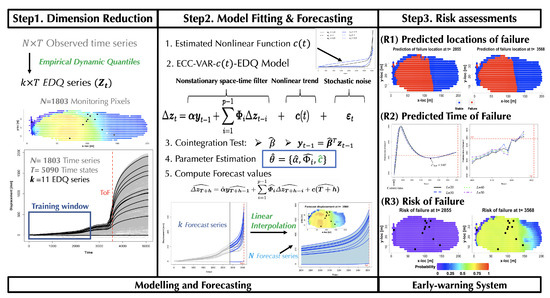
Figure 2.
Overview of the forecasting framework. There are two parts of this forecasting framework. The first part is modelling and forecasting. The second part is building an early-warning system to predict future failure with three risk assessments (R1–R3).
In step 1, we first apply a dimension reduction technique to reduce the dimension of the large-scale dataset from to a small number k, which can make sure computation ia feasible for the further steps in our method, with a negligible loss of spatial and temporal dynamical information. We use the training sample to identify these k locations from the entire domain (i.e., with for Slope X data for purpose of illustration). To achieve this, we apply the idea of empirical dynamic quantiles (EDQ), introduced by [12] and first used in a forecasting model for high-dimensional landslides data in [14]. The key idea behind this technique is that the dimension reduction to k EDQ series at k quantile levels is achieved by selecting a small subset series from the original observed time series set, which is able to retain the dynamic dependence in the original dataset. This small set time series selected at k quantile levels optimally represents the whole time series set. Note that finding the k EDQ series from the original time series set is the same as finding the k locations from the 1803 monitoring locations. Statistical computations used to determine the k representative EDQ series essentially involve minimizing the sum of absolute differences between each observed time series and the prospective EDQ series at the given quantile level. This optimization procedure is computationally feasible and statistically consistent; more details ar eprovided in [12]. These k representative EDQ series enable us to perform various statistical inferences and forecasting in a manner that captures and retains the essential spatial–temporal dynamics that drive the slope’s surface motion as damage spreads in the landslides. Similarly, the quantile level for each location and time series in the training data can also be determined by this technique.
In step 2, we develop a model using the training sample from the representative k EDQ series to capture the nonstationary, nonlinear trends and spatial–temporal dynamics in the ground motion system. It is important to have such a model to provide reliable and timely forecasts for this complex system. Unlike most existing time-series forecasting methods [7,8,11], our model considers both the nonstationary and nonlinear observed time series. To develop such a model, we use the concepts of vector autoregression (VAR) time series and error-correction cointegration (ECC) modelling [15,16] to deal with the nonstationarity and combine these with an empirical function in terms of time t to capture the nonlinear trends in the ground motion system. We call this method the ECC-VAR--EDQ model. Let be the k dimension vector time series of displacement observed from k EDQ locations, and be the velocity. The key equation for this ECC-VAR--EDQ model is of the following form
where , with being the co-integration matrix of rank r; is the stationary adjustment matrix, which is also of rank r; s are the space–time association matrices; is the predefined function of time t used to capture the nonlinearity; is a sequence of independent and identically distributed k random vectors with mean zero and covariance matrix . Determining model (1) and estimating the parameters are the tasks undertaken in step 2 of Figure 2.
The first key property of Equation (1) contains a valid analysis of the nonstationary, spatial–temporal dynamics, where is usually nonstationary in real-world dataset [8] but must be stationary if is stationary. Here, we apply the idea of cointegration [17,18,19]—a linear combination of these k unit-root nonstationary time series that become r stationary series . The linear combination matrix is called a cointegrating matrix with rank r. Cointegration implies a long-term stable relationship between variables in forecasting [15]. Another important feature of Equation (1) is its capacity for nonlinearity in the function . A broad exploration and the literature show that empirical approaches are quite often used to overcome the difficulties encountered when using the nonlinear theoretical formulations [20,21]. Here, we use an empirical method to determine -employ the flexible mathematical functions and represent the nonlinear trend by adapting parameters.
Specifically, to fit and estimate this model (1), we need to determine the cointegration rank r and the cointegration matrix . Consider the ECC-VAR--EDQ model (1) and replace ; then, we have
where . The matrix plays an important role in the cointegration study: if , there is no cointegrating vector. In other words, the test for cointegration focuses on testing the rank of matrix . Johansen’s method is the best-known cointegration test for VAR models; see more details in [22,23]. Impact matrix is the coefficient of the lagged levels in a nonlinear least squares regression of on lagged differences and lagged levels and function [15,17]. Three main steps are used to test the rank of the impact matrix : since is related to the covariance matrix between and , the mean will not influence the estimation of . We can first simplify the Equation (2) by concentrating on the effect of the lagged differences and function . Let us achieve this by first regressing on function and the lagged differences , providing the residuals and then regressing on function and the lagged differences , leading to the residuals as Equation (3). After performing these two regressions, we obtain the simplified model as Equation (4).
where is our pre-defined function to capture the nonlinear trend. These two regressions in Equation (3) can be estimated by the least-squares (LS) method and are the residuals obtained from these two regressions. Then, we have the simplified model as follows,
The least-squares estimate of matrix is identical for Equation (2) and the simplified model (4). Hence, testing the rank of the covariance matrix between the and is equivalent to testing the rank of the covariance matrix between and . We can focus on testing the rank of the matrix in Equation (4). We use the likelihood ratio test (LRT) to test the rank of and find the estimated cointegrating vector . Let
be the nested models such that, under , there are r cointegrating vectors in . In particular, under we have . Under rank; that is, there are r linearly independent vectors among these k vectors and the maximum likelihood estimate (MLE) of is
The maximized likelihood function is, therefore, approximate to
Under rank, that is, the matrix is full rank, there is no constraint on the covariance matrix. Similarly, we can obtain the maximized likelihood function under and the likelihood ratio is, therefore,
We define
Then, the sample matrix becomes and be the ordered eigenvalues of the sample matrix and be the eigenvector associated with eigenvalue Here, are the eigenvalues of . We can obtain the likelihood ratio test statistic as follows
Reject the null hypothesis if is larger than the critical value and the estimated cointegrating vector can be obtained from the r corresponding eigenvectors [17,18].
Another aspect of fitting and estimating the ECC-VAR--EDQ model (1) is the determination of . Johansen also pointed out that the function in Equation (2) has important implications in a cointegrated system [24]. Tavenas and Leroueil pointed out that the rationale for most time-of-failure predictions is that the slope displacement can be represented by a creep curve before rupture [25], which can be divided into three stages. According to the classic interpretation, the first stage is primary creep, with the strain rate decreasing logarithmically, followed by secondary (or steady-state) creep with a constant strain rate, and tertiary creep with an increasing creep rate, which leads to rupturing. Our aim was to capture the nonlinear trend by using a function that is equivalent to finding a method to represent the creep curves. Empirical methods have been used extensively to represent creep curves, which requires a user to define the functions to represent the curve models from the data trend [26,27]. Research and experiments have found that it is sufficient to obtain an accurate representation of the creep curve by adding the primary part and tertiary part together [21,28]. At present, these empirical approaches use the simple power function combined with exponential function to represent the creep curves [21,28,29]. Here, we apply the empirical method to determine the form of function . Let have the form of where is used to capture the trend in precursory failure regime and is used to capture the nonlinear trend in tertiary creep. Then, the deterministic function has the following form:
where are the pre-estimated parameters for the form of obtained by using penalized maximum likelihood; is the time state, which can be determined by prior work. When , then will mainly be influenced by ; on the other hand, when will have an exponential growth, and will mainly be influenced by , which can be used to represent the creep curve. Figure 3 provides several examples of with different values of .
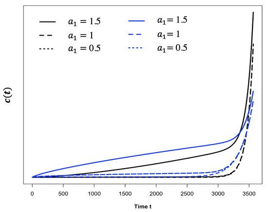
Figure 3.
Curve of function with different values of . The black lines are with three different values of . The blue lines are with three different values of .
We use the cointegration test with our pre-estimated function finding the estimated cointegrating matrix . After that we can fit and estimate the ECC()-VAR(p)--EDQ model (1) with . We use least square (LS) method estimate the unknown parameters , is the parameters from function. Once we have the fitted model, we can calculate the forecast values of the k EDQ displacement series at times and beyond. The forecast values and can be denoted as and ; at future time steps, are
where and if (i.e., if t is inside the training data), and are the estimated parameters in model (1). We then employ these forecast results to interpolate and approximate the displacement in the other locations at future time. For example, to forecast the displacement at location i with EDQ quantile level at time , we first figure out the two adjacent quantile levels and from the k EDQ series we found in part 1 with their forecast displacement and , such that . Then, can be calculated by
In step 3, once we obtain the forecast displacement across the entire domain, we can provide predictions for where and when a future failure will occur by using three risk assessments in parallel. The first uses the clustering method for the forecast values at all locations at a specific future time states to determine the likely locations of failure. The second one uses the adaptive Fukuzono method on the EDQ time series to estimate the earliest time of failure (ToF), which is more objective than traditional Fukuzono regression. The last one delivers a spatial map of the probability of risk of failure at each future time steps, which is calculated by the prescribed what-if-scenario (e.g., a scenario when the forecast velocity at a location exceeds a predefined threshold value). Details will be provided in Section 5 by analyzing the Slope X data described in Section 2.
4. Apply to Slope X Data
To assess the performance of our ECC(r)-VAR(p)--EDQ model, we applied it to real-world slope data. It is common to split the dataset into two parts when developing statistical and machine learning models [30,31]. Many researchers proposed a ratio of 80/20 for producing a training/testing dataset for landslide susceptibility problems [32,33]. The other principle for determining the training data is that they must not contain the actual failure but should contain some information on precursory failure. Therefore, we used the training set with length of Slope X data, starting from to , and used the data starting from to (the actual time of failure) as our test sample ( of the observed data). There was no issue regarding which part was used as the training sample; to prove this, we also provide the results obtained when using moving training samples in Section 5. As Section 3 describes, first, we selected the EDQ series to represent the entire time series based on the training sample. These 11 EDQ series at quantile levels- with the corresponding monitoring pixel ID are . The displacement and locations for these 11 EDQ series are highlighted in black in Figure 1. We used the training sample to fit and estimate the ECC(r)-VAR(p)--EDQ model.
In Figure 3, the black solid is shown capture the shape of creep curve well; therefore, we chose the empirical function to represent the nonlinear trend. Based on the current knowledge from the data, when , there is some acceleration trend; therefore, here, we took the current estimated time of failure as prior . Next, we applied the cointegration test described in Section 3 for the 11 EDQ series . The test results conclude that for the Slope X data. A goodness of fit test using coefficient of determination shows that an auto-regression order of is sufficient for modelling the Slope X data. Eventually, we determined the optimal values for all unknown parameters in ECC(8)-VAR(2)--EDQ model (1). The forecast displacements for the 11 selected EDQ locations at the test sample times are displayed in Figure 4.
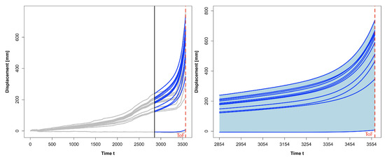
Figure 4.
(Left) For the 11 selected EDQ series; (Right) for all 1803 time series. Forecast displacement at time to based on the training sample starting from to . The red dashed line is the actual time of failure at .
These forecasts overall conform to the increasing trends of the observed displacement data (the grey curves in the plot). Such an observation is expected and was invariant to the selection of training data according to the established properties underlying the current vector time series forecasting methods. Clearly, the forecasts for each EDQ location are mostly greater than the actual observations, except when t is very close to the actual failure time (). Apart from the 11 selected EDQ series, forecast displacement for the remaining 1792 time series over time was computed using Equation (11). The results for the displacement forecasts are displayed in the right plot of Figure 4. These displacement forecasts can also be depicted as a heat map for each future time t. Such a heat map, at and , is displayed in Figure 5, along with its histogram plot.
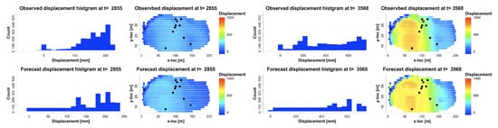
Figure 5.
Forecast displacement at all these 1803 monitoring pixels. (Left) forecast displacement at ; (Right) forecast displacement at , ToF.
5. Results and Discussion
Here, we built an early-warning system to predict the locations, time and risk of a future failure using three risk assessments. These risk assessments were based on the forecast values and provide more objective assessments. The results of these risk assessments apply to the forecast values for slope X data, and are shown in Figure 6, Figure 7 and Figure 8.
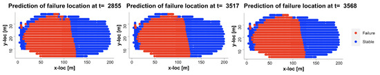
Figure 6.
(R1) Predicted locations of failure using clustering at time .
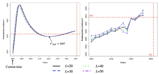
Figure 7.
(R2) Predicted time of failure using adaptive Fukuzono analysis. The left plot is for fixed training data with rolling Fukuzono regression window. The right plot is for the rolling training sample with fixed Fukuzono regression window.
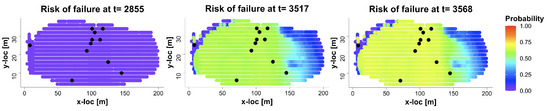
Figure 8.
(R3) predicted risk of failure for what-if-scenario at time .
The first risk assessment (R1) focuses on identifying the likely locations of the slope failure. This can be achieved by using the displacement forecasts to cluster all monitoring locations into stable and failure regions for each future time t. We used the simple K-means clustering to perform such a clustering for Slope X data [34,35] (e.g., K = 2 clusters, for stable and failure). From Figure 6, we can clearly identify the predicted failure pattern from , the first time state at our forecast horizon (i.e., 2 days, 23:18 to ToF), and this failure geometry remains unchanged as the forecast time state moves forward until (ToF).
The second risk assessment (R2) focuses on predicting the time of failure (ToF) by using an adaptive Fukuzono method for the forecasts of each selected EDQ series. The classical Fukuzono method draws a regression line based on selected observed inverse velocities and extends the regression line forward until it intersects with the time axis, and the intersection is the Fukuzono estimated time of failure [36]. This method depends on (1) the start location and (2) the number of inverse velocities used for regression. Instead of determining these two things by personal choice or some prior work, here, we improved the Fukuzono method by using a more objective method. As the left panel in Figure 7 shows, we applied a moving Fukuzono regression window to the forecast timeline with different sizes: . Each curve represents the predicted time of failure using one Fukuzono regression window with size L at different time states. For example, the black lines is the obtained from the moving Fukuzono regression window with length L towards the forecast horizon for the Max quantile EDQ series. The intersection of these four curves will be treated as the convergence point of the predicted time of failure. Figure 7 shows that our predicted time of failure is , which is 8 h before the actual time of failure. We also assessed the performance of our model (1) using a moving training window. As the right plot in Figure 7 shows, there are 14 different training samples in total; we used the training sample starting at time interval and then moved forward by 50 with a fixed length 2854. Based on each training window, we used the first L forecasts to find the Fukuzono regression and obtain the predicted time of failure. Figure 7 shows that when the training window is closer to the actual ToF, our predicted ToF will be closer to the actual time of failure, with the minimum error of h before the actual ToF.
The third risk assessment (R3) focuses on the risk of failure in terms of quantified uncertainty under a given what-if-scenario. In general, the risk of failure is a probability function of certain measured slope feature, aiming to reach a threshold hazard level at a future time state [37]. Our task is to generate a spatial map of the risk of failure for every monitoring location and every future time state until the actual failure occurs. For example, slope motion velocity data exceeding 10 mm/h mm/6 min are understood as dangerous, prompting an immediate red-alert warning [38]. Then, we can calculate the risk of failure for Slope X data for location i from time to 3568. As Figure 8 shows, we can identify the time for each location when the forecast risk of failure exceeds 60% probability. For example, for the level-1.0 EDQ location when , 5.1 h before the actual time of failure . It should be noted that these risk-of-failure results are obtained using the observations from to , about 71.4 h before the actual landslide. Therefore, we can conclude that our ECC-VAR--EDQ method is able to accurately predict an impending landslide, by providing a or more risk of rock failure for each location, more than 71 h in advance. The spatial map of risks of failure at time and all monitoring locations are displayed in Figure 8. All the findings from Figure 6, Figure 7 and Figure 8 show that this assessment is capable of providing timely and accurate ToF estimates.
6. Conclusions
We developed a statistical model and an early-warning system to forecast landslides. This ECC-VAR--EDQ model is computationally feasible and comprehensive to deal with high-dimensional, spatial–temporal-dependent time series with nonlinear and nonstationary phenomena. The results of the application of this ECC-VAR--EDQ model fitted the real-world Slope X data () and provided reliable early-warning predictions for decision-making and risk mitigation. Finally, there is still some further work that could improve our proposed ECC-VAR--EDQ model. For example, we used empirical functions to represent the nonlinear trend , they are generally faster and straightforward to use, but make stronger assumptions about the parameters of the data distribution of time series; hence, non-parametric methods can be considered for further work.
Author Contributions
Conceptualization, G.Q. and A.T.; methodology, G.Q. and H.Z.; software, H.Z.; validation, H.Z., G.Q. and A.T.; formal analysis, H.Z. and G.Q.; investigation, H.Z.; data curation, A.T.; writing—original draft preparation, H.Z.; writing—review and editing, H.Z. and G.Q.; visualization, H.Z.; supervision, G.Q. and A.T.; funding acquisition, A.T. All authors have read and agreed to the published version of the manuscript.
Funding
This research was partly funded by the U.S. DoD High Performance Computing Modernization Program (HPCMP) and RDECOM International Technology Center-Pacific (ITC-PAC) contract number: FA5209-18-C-0002.
Institutional Review Board Statement
Not applicable.
Informed Consent Statement
Not applicable.
Data Availability Statement
The landslide data analyzed in this study is confidential and is subject to a non-disclosure agreement between the University of Melbourne and an undisclosed industry partner. Simulated data are available on request from the corresponding author.
Acknowledgments
The authors thank the ITISE 2023 Organization and the two anonymous reviewers for providing valuable comments and suggestions, leading to an improvement of the presentation of the paper.
Conflicts of Interest
The authors declare no conflict of interest.
References
- Uhlemann, S.; Smith, A.; Chambers, J.; Dixon, N.; Dijkstra, T.; Haslam, E.; Meldrum, P.; Merritt, A.; Gunn, D.; Mackay, J. Assessment of Ground-based Monitoring Techniques Applied to Landslide Investigations. Geomorphology 2016, 253, 438–451. [Google Scholar] [CrossRef]
- Zhao, C.; Lu, Z. Remote Sensing of Landslides—A Review. Remote Sens. 2018, 10, 279. [Google Scholar] [CrossRef]
- Chuvieco, E. Fundamentals of Satellite Remote Sensing: An Environmental Approach; CRC Press: Boca Raton, FL, USA, 2016. [Google Scholar]
- Riley, K.; Webley, P.; Thompson, M. Natural Hazard Uncertainty Assessment: Modeling and Decision Support; John Wiley & Sons: Hoboken, NJ, USA, 2016. [Google Scholar]
- Dick, G.J.; Eberhardt, E.; Cabrejo-Liévano, A.G.; Stead, D.; Rose, N.D. Development of an Early-warning Time-of-failure Analysis Methodology for Open-pit Mine Slopes Utilizing Ground-based Slope Stability Radar Monitoring Data. Can. Geotech. J. 2015, 52, 515–529. [Google Scholar] [CrossRef]
- Kumar, C.; Patel, N.; Jaudi, I. 21st Century Physics: Grand Challenges. J. Fed. Am. Sci. 2003, 56, 9–11. [Google Scholar]
- Aggarwal, A.; Alshehri, M.; Kumar, M.; Alfarraj, O.; Sharma, P.; Pardasani, K.R. Landslide Data Analysis Using Various Time Series Forecasting Models. Comput. Electr. Eng. 2020, 88, 106858. [Google Scholar] [CrossRef]
- Cheng, C.; Sa-Ngasoongsong, A.; Beyca, O.; Le, T.; Yang, H.; Kong, Z.; Bukkapatnam, S. Time Series Forecasting for Nonlinear and Non-stationary Processes: A Review and Comparative Study. Iie Trans. 2015, 47, 1053–1071. [Google Scholar] [CrossRef]
- Tien Bui, D.; Tuan, T.A.; Klempe, H.; Pradhan, B.; Revhaug, I. Spatial Prediction Models for Shallow Landslide hazards: A comparative assessment of the efficacy of support vector machines, artificial neural networks, kernel logistic regression, and logistic model tree. Landslides 2016, 13, 361–378. [Google Scholar] [CrossRef]
- Salles, R.; Belloze, K.; Porto, F.; Gonzalez, P.H.; Ogasawara, E. Nonstationary Time Series Transformation Methods: An Experimental Review. Knowl.-Based Syst. 2019, 164, 274–291. [Google Scholar] [CrossRef]
- De, G.; Jan, G.; Hyndman, R.J. 25 Years of Time Series Forecasting. Int. J. Forecast. 2006, 22, 443–473. [Google Scholar]
- Peña, D.; Tsay, R.S.; Zamar, R. Empirical Dynamic Quantiles for Visualization of High-dimensional Time Series. Technometrics 2019, 61, 429–444. [Google Scholar] [CrossRef]
- Tordesillas, A.; Kahagalage, S.; Campbell, L.; Bellett, P.; Intrieri, E.; Batterham, R. Spatiotemporal Slope Stability Analytics for Failure Estimation (SSSAFE): Linking Radar Data to the Fundamental Dynamics of Granular Failure. Sci. Rep. 2021, 11, 1–18. [Google Scholar] [CrossRef]
- Wang, H.; Qian, G.; Tordesillas, A. Modeling Big Spatio-temporal Geo-hazards Data for Forecasting by Error-correction Cointegration and Dimension-Reduction. Spat. Stat. 2020, 36, 100432. [Google Scholar] [CrossRef]
- Tsay, R.S. Multivariate Time Series Analysis: With R and Financial Applications; John Wiley & Sons: Hoboken, NJ, USA, 2013. [Google Scholar]
- Sa-Ngasoongsong, A.; Bukkapatnam, S.T.S.; Kim, J.; Iyer, P.S.; Suresh, R.P. Multi-step Sales Forecasting in Automotive Industry Based on Structural Relationship Identification. Int. J. Prod. Econ. 2012, 140, 875–887. [Google Scholar] [CrossRef]
- Johansen, S. Statistical Analysis of Cointegration Vectors. J. Econ. Dyn. Control 1988, 12, 231–254. [Google Scholar] [CrossRef]
- Reinsel, G.C.; Ahn, S.K. Vector Autoregressive Models with Unit-roots and Reduced Rank Structure: Estimation. Likelihood Ratio Test, and Forecasting. J. Time Ser. Anal. 1992, 13, 353–375. [Google Scholar] [CrossRef]
- Pfaff, B. Analysis of Integrated and Cointegrated Time Series with R; Springer Science & Business Media: Berlin/Heidelberg, Germany, 2008. [Google Scholar]
- Hadid, M.; Rechak, S.; Tati, A. Long-term Bending Creep Behavior Prediction of Injection Molded Composite Using Stress–Time Correspondence Principle. Mater. Sci. Eng. A 2004, 385, 54–58. [Google Scholar] [CrossRef]
- Sandström, R. Basic Model for Primary and Secondary Creep in Copper. Acta Mater. 2012, 60, 314–322. [Google Scholar] [CrossRef]
- Johansen, S.; Juselius, K. Maximum Likelihood Estimation and Inference on Cointegration—With Appucations to the Demand for Money. Oxf. B Econ. Stat. 1990, 52, 169–210. [Google Scholar] [CrossRef]
- Johansen, S. Estimation and Hypothesis Testing of Cointegration Vectors in Gaussian Vector Autoregressive models. Econ. J. Econ. Soc. 1991, 59, 1551–1580. [Google Scholar] [CrossRef]
- Johansen, S. Likelihood-Based Inference in Cointegrated Vector Autoregressive Models; Oxford University Press: Oxford, UK, 1995. [Google Scholar]
- Tavenas, F.; Leroueil, S. Creep and Failure of Slopes in Clays. Can. Geotech. J. 1981, 18, 106–120. [Google Scholar] [CrossRef]
- Abdallah, Z.; Gray, V.; Whittaker, M.; Perkins, K. A Critical Analysis of the Conventionally Employed Creep Lifing Methods. Materials 2014, 7, 3371–3398. [Google Scholar] [CrossRef] [PubMed]
- Gray, V.; Whittaker, M. Development and Assessment of a New Empirical Model for Predicting Full Creep Curves. Materials 2015, 8, 4582–4592. [Google Scholar] [CrossRef] [PubMed]
- Yang, L.; Li, Z. Nonlinear Variation Parameters Creep Model of Rock and Parametric Inversion. Geotech. Geol. Eng. 2018, 36, 2985–2993. [Google Scholar] [CrossRef]
- Sattar, M.; Othman, A.R.; Kamaruddin, S.; Akhtar, M.; Khan, R. Limitations on the Computational Analysis of Creep Failure Models: A Review. Eng. Fail. Anal. 2022, 134, 105968. [Google Scholar] [CrossRef]
- Nguyen, Q.H.; Ly, H.B.; Ho, L.S.; Al-Ansari, N.; Le, H.V.; Tran, V.Q.; Prakash, I.; Pham, B.T. Influence of Data Splitting on Performance of Machine Learning Models in Prediction of Shear Strength of Soil. Math. Probl. Eng. 2021, 2021, 1–15. [Google Scholar] [CrossRef]
- Joseph, V.R.; Vakayil, A. Split: An Optimal Method for Data Splitting. Technometrics 2022, 64, 166–176. [Google Scholar] [CrossRef]
- Chen, W.; Peng, J.; Hong, H.; Shahabi, H.; Pradhan, B.; Liu, J.; Zhu, A.; Pei, X.; Duan, Z. Landslide Susceptibility Modelling Using GIS-based Machine Learning Techniques for Chongren County, Jiangxi Province, China. Sci. Total Environ. 2018, 626, 1121–1135. [Google Scholar] [CrossRef]
- Pham, B.T.; Tien Bui, D.; Pourghasemi, H.R.; Indra, P.; Dholakia, M.B. Landslide Susceptibility Assesssment in the Uttarakhand area (India) using GIS: A Comparison Study of Prediction Capability of Naïve Bayes, Multilayer Perceptron Neural Networks, and Functional Trees Methods. Theor. Appl. Climatol. 2017, 128, 255–273. [Google Scholar] [CrossRef]
- Kodinariya, T.M.; Makwana, P.R. Review on Determining Number of Cluster in K-Means Clustering. Int. J. 2013, 1, 90–95. [Google Scholar]
- Likas, A.; Vlassis, N.; Verbeek, J.J. The Global K-means Clustering Algorithm. Pattern Recognit. 2003, 36, 451–461. [Google Scholar] [CrossRef]
- Fukuzono, T. A Method for Predicting the Failure Time of a Sandy Soil Slope using the Inverse Number of Velocity. In Proceedings of the 23rd Meeting of Japan Landslide Society, Tokyo, Japan, 2 July 1984; pp. 80–81. [Google Scholar]
- Wang, R.; Li, L.; Simon, R. A Model for Describing and Predicting the Creep Strain of Rocks from the Primary to the Tertiary Stage. Int. J. Rock Mech. Min. Sci. 2019, 123, 104087. [Google Scholar] [CrossRef]
- Mufundirwa, A.; Fujii, Y.; Kodama, J. A New Practical Method for Prediction of Geomechanical Failure-time. Int. J. Rock Mech. Min. Sci. 2010, 47, 1079–1090. [Google Scholar] [CrossRef]
Disclaimer/Publisher’s Note: The statements, opinions and data contained in all publications are solely those of the individual author(s) and contributor(s) and not of MDPI and/or the editor(s). MDPI and/or the editor(s) disclaim responsibility for any injury to people or property resulting from any ideas, methods, instructions or products referred to in the content. |
© 2023 by the authors. Licensee MDPI, Basel, Switzerland. This article is an open access article distributed under the terms and conditions of the Creative Commons Attribution (CC BY) license (https://creativecommons.org/licenses/by/4.0/).