Light Sheet Fluorescence Microscopy Using Incoherent Light Detection ^†

Abstract

We previously developed an incoherent holography technique for use in lattice light sheet (LLS) microscopes that represents a specialized adaptation of light sheet microscopy. Light sheet instruments resolve 3D information by illuminating the sample at 90° to the imaging plane with a sheet of laser light that excites fluorophores in the sample only in a narrow plane. Imaging this plane and then moving it in the imaging z-axis allows construction of the sample volume. Among these types of instruments, LLS microscopy gives higher z-axis resolution and tissue depth penetration. It has a similar working principle to light sheet fluorescence microscopy but uses a lattice configuration of Bessel beams instead of Gaussian beams. Our incoherent light detection technique replaces the glass tube lens of the original LLS with a dual diffractive lens system to retrieve the axial depth of the sample. Here, we show that the system is applicable to all light sheet instruments. To make a direct comparison in the same emission light path, we can imitate the nature of non-Bessel light sheet systems by altering the mask annuli used to create Bessel beams in the LLS system. We change the diffractive mask annuli from a higher NA anulus to a smaller NA anulus. This generates a Gaussian excitation beam similar to conventional light sheet systems. Using this approach, we propose an incoherent light detection system for light sheet 3D imaging by choosing a variable NA and moving only the light sheet while keeping the sample stage and detection microscope objective stationary.

1. Introduction

Continuous irradiation causes photodamage and phototoxicity when imaging living samples and specimens. In order to overcome this problem, light sheet fluorescence microscopy (LSFM) was developed as an imaging technique with good optical sectioning, to record faster and scan larger sample volumes at low radiation intensities over longer time frames [1]. The LSFM is similar to laser scanning confocal microscopy (LSCM) [2], but the emitted fluorescence light is collected by the detection objective in a perpendicular direction from the excitation light and without the need for a confocal aperture. In LSFM, the excitation light does not pass through the entire sample; instead, the sample is illuminated from the side with a thin light sheet (LS) beam. This clever idea allows the LSFM to collect the emitted light from fluorophores localized in the thin LS plane only and not from fluorophores belonging outside the LS plane. This results in a low light dose usage, and therefore reduces both photobleaching and phototoxicity [3,4,5]. LSFM is also referred to as selective-plane illumination microscopy (SPIM) when imaging large samples [1]. The axial resolution is given by both the thickness of the LS (ideally it is extremely thin) and the detection NA [6,7]. If we choose a microscope objective with an NA of 1.1, we can obtain a very thin light sheet. However, the light sheet confocal length, over which the sheet is thin, must be matched to the FOV of the recorded images or the size of the samples. The thinner the sheet (and higher the NA), the shorter the thin region is.

In most of the cases, the light sheet has a Gaussian profile at the specimen due to the Gaussian shape of the laser beams. A thicker Gaussian light sheet can cover a larger FOV but has a lower resolution and optical sectioning. Non-Gaussian beams using arrays of Bessel beams, called “lattice” beams, have been employed to generate images with excellent scanning efficiency and resolution, by using very thin light sheets. The lattice light sheet microscopy (LLSM) system uses the LSFM principle with an optical lattice created with Bessel beams, resulting in a light sheet with a thickness of ~400 nm [8]. The typical acquisition rate of an LLSM system is hundreds of frames per second, making LLSM the ultimate tool for live-cell fluorescence imaging.

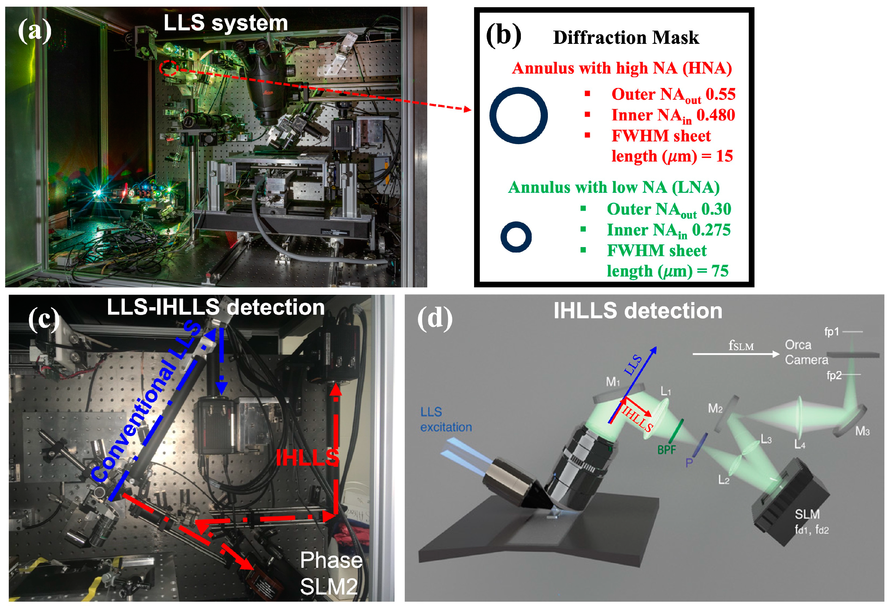
The lattice light sheet, Figure 1a, is formed by superimposing a linearly polarized sheet of light with a binary phase map of Bessel beams on a binary spatial light modulator (SLM), which is conjugated to the image plane of the excitation objective. Before reaching the sample plane, the beam passes a Fraunhofer lens and is further projected onto a transparent optical annulus, Figure 1b, to eliminate unwanted diffraction orders and lengthen the light sheet. In dithered mode, a 2D lattice pattern is oscillated in the x-axis using a galvanometer (x-galvo), to create a uniform sheet, while another galvanometer mirror moves together with the detection objective, in the z-axis (z-galvo), to scan the sample volume.

A more recent approach of the LLSM is the new detection path, Figure 1c,d, that uses the incoherent holography idea, called an incoherent holographic lattice light sheet (IHLLS) [9], to scan the sample volume without moving the detection objective. It is possible by projecting two diffractive lenses at various z-galvo positions, using a phase SLM, to encode the depth position of the sample being imaged. The annular mask, Figure 1b, mentioned above, was centered on an anulus with a higher NA (HNA), NAout = 0.5, NAin = 0.485, and a sheet length 15 μm; therefore, the beams used for excitation were more Bessel-like beams. The intensity profile of the obtained optical lattice is determined by both the applied binary phase map and the geometry of the transparent annulus.

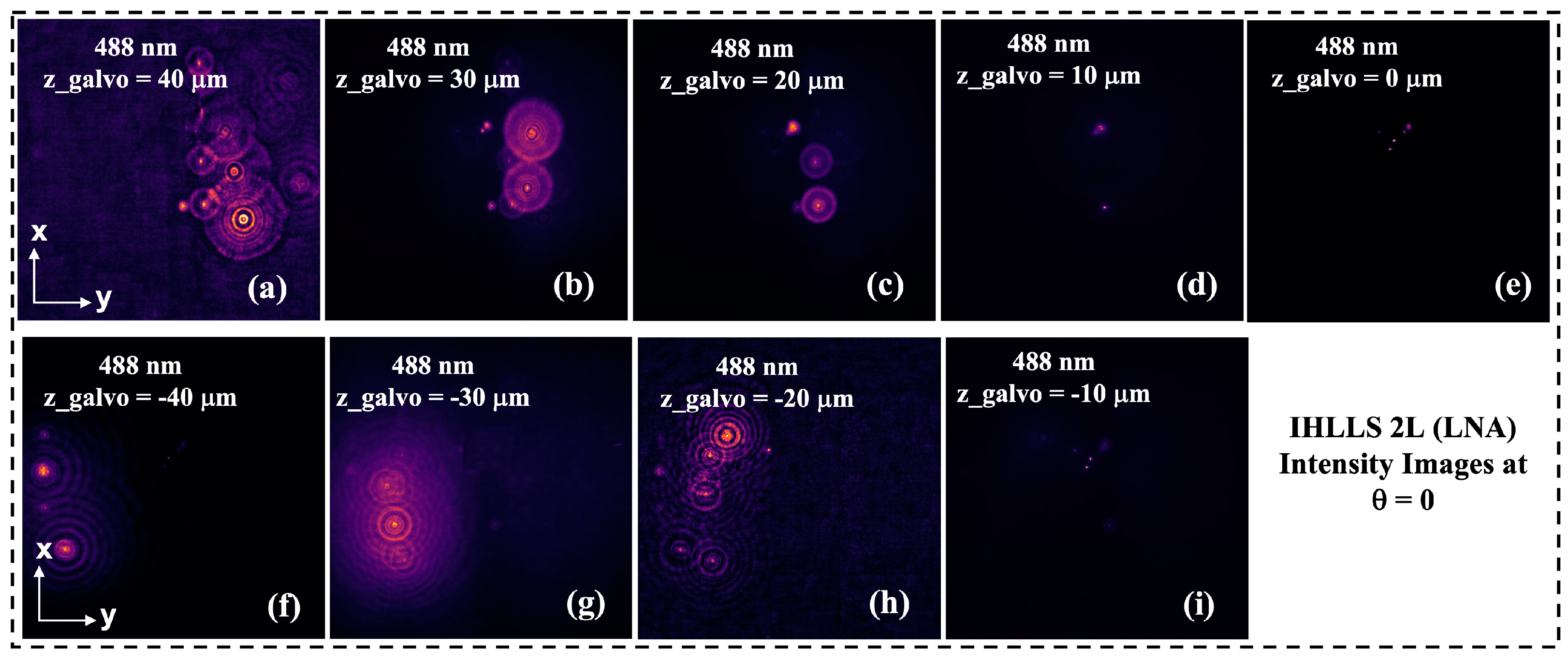
Here, we propose to expand our previous IHLLS detection technique that uses a HNA by choosing a diffractive mask annulus with a lower NA (LNA). In this case, the anulus has the following parameters: NAout = 0.3, NAin = 0.275, and sheet length 75 μm. The new detection approach uses a Gaussian-like excitation beam similar to conventional light sheet systems. This provides a tradeoff between the size of the imaged beam and the resolution of the ultimate image in the z-plane. This has advantages for imaging objects at larger intercellular scales.

2. Imaging Performances and Diffraction Mask Parameter Selection

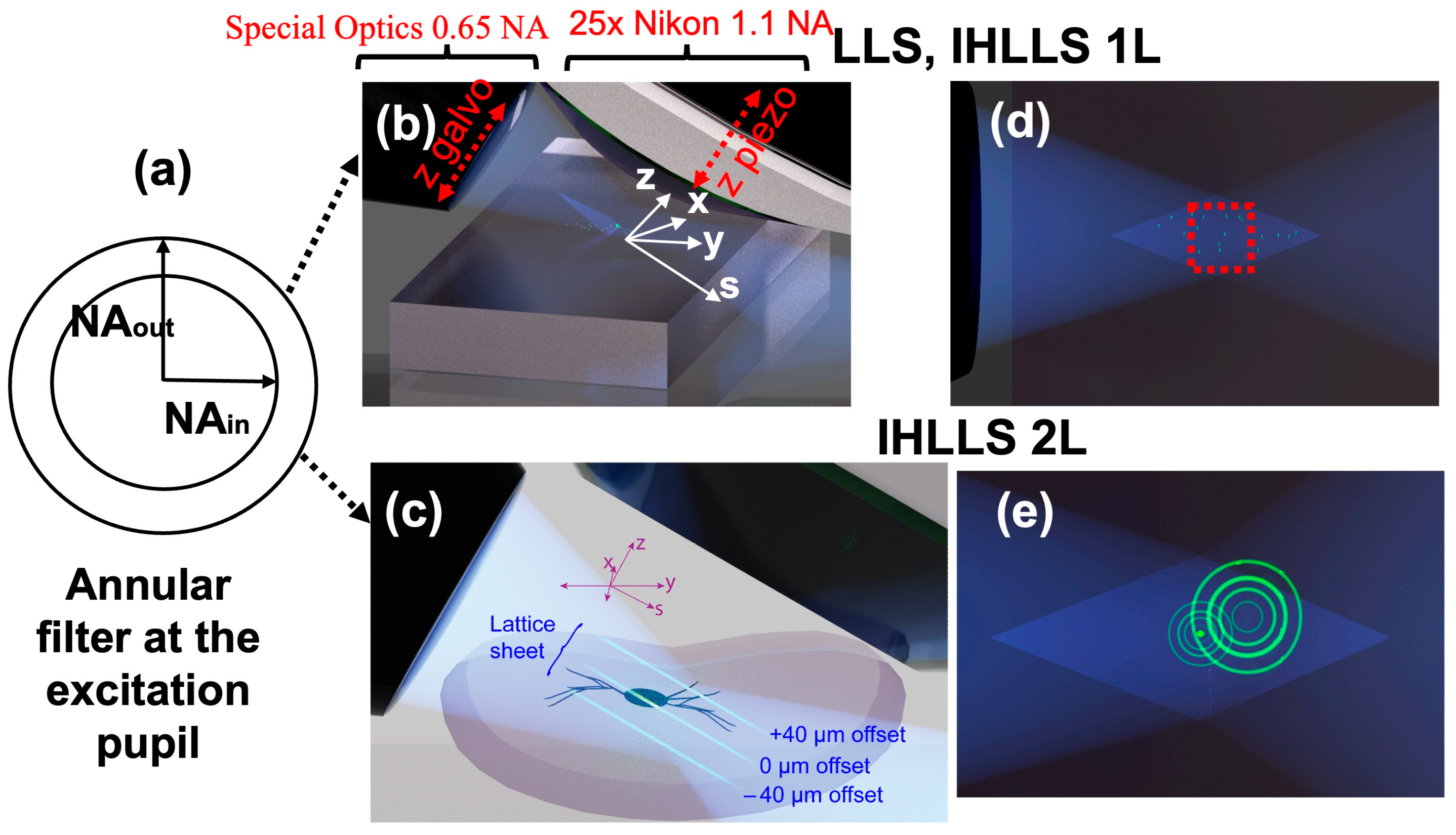
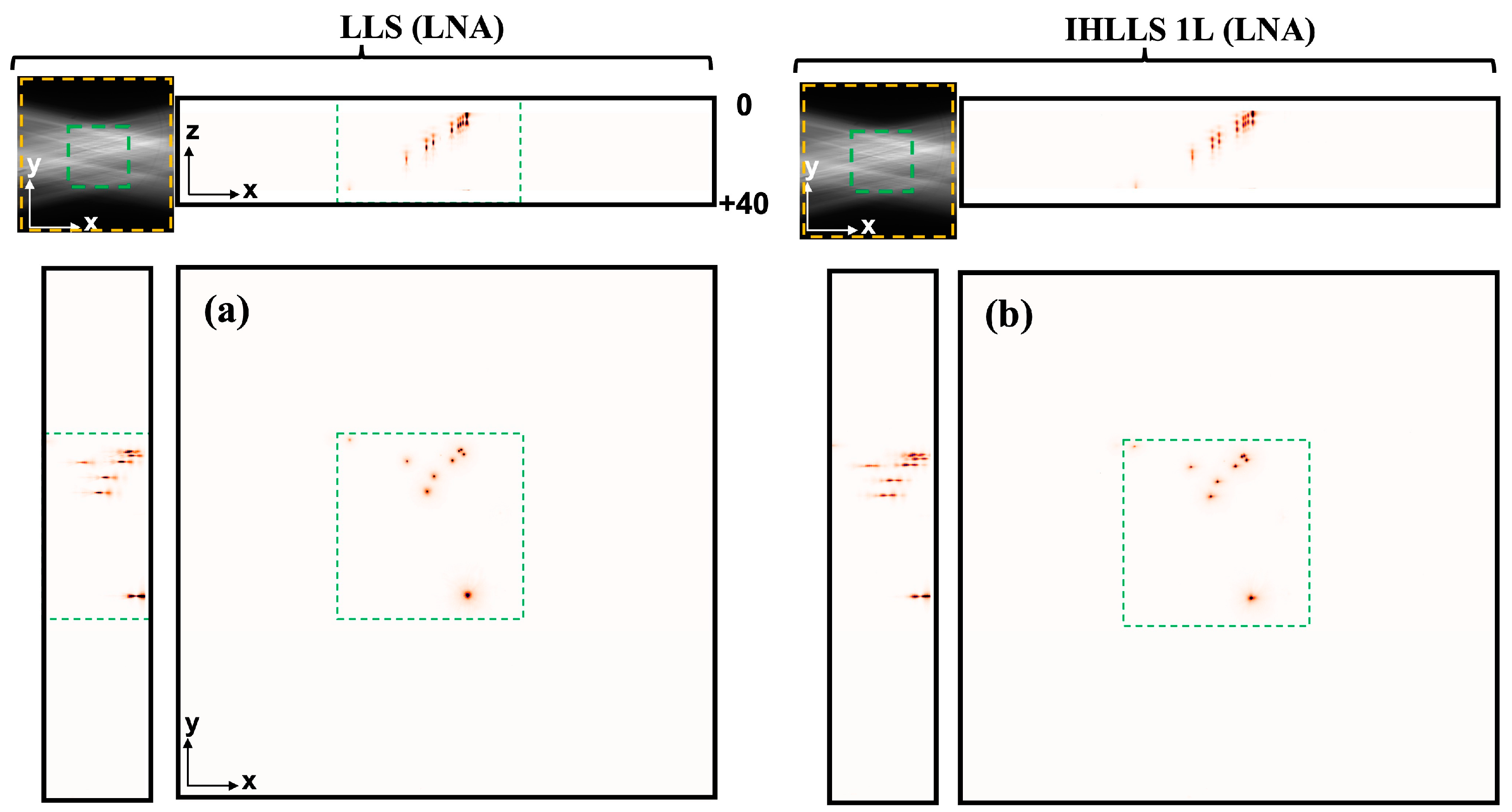
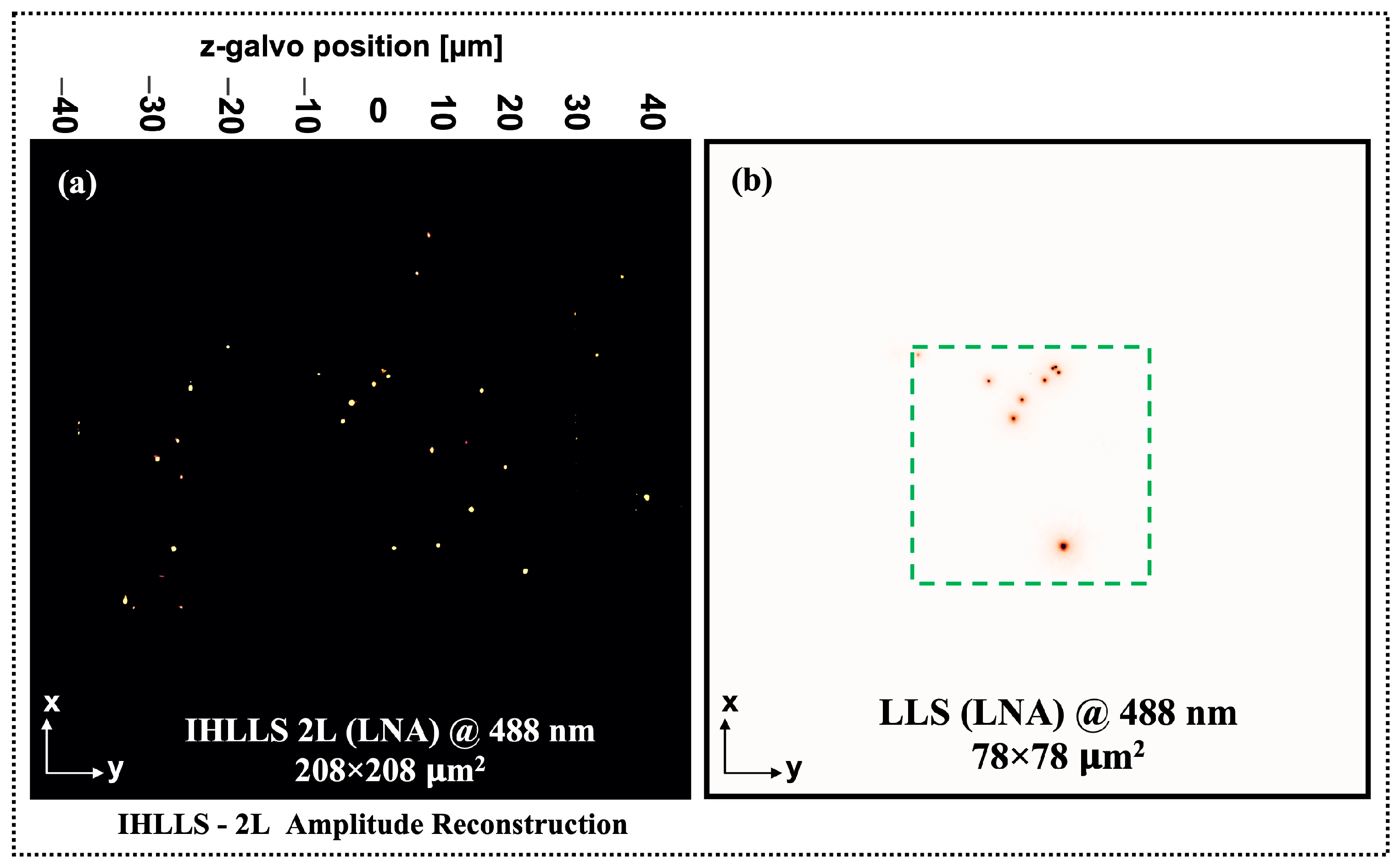
In LLS, near-non-diffracting Bessel beams are created at the focal position of the excitation objective, by projecting an annular excitation beam, Figure 2a, in the back focal plane of the excitation objective. While the z-galvo and z-piezo are moved along the z axis to acquire stacks in LLS/IHLLS 1L, Figure 2b, in IHLLS 2L only the z-galvo is moved at various z positions, Figure 2c. The imaging area/volume is limited to a small FOV, Figure 2d red square, due to the tradeoff between the sheet’s propagation length and its thickness. Although IHLLS 1L is the incoherent version of the LLS detection module, the axial resolution in LLS is better than the axial resolution in IHLLS 1L due to the blurry effect of the diffractive lens that focusses to infinity. The FOV limitation is no longer an issue in IHLLS 2L because the combination of the z-galvo motion in the range $-40\mathsf{\mu }\mathrm{m}\mathrm{t}\mathrm{o}+40\mathsf{\mu }\mathrm{m}$ and the dual diffractive lenses uploaded onto the phase SLM allows scanning for the whole FOV of the CMOS detector, which is 208 × 208 ${\mathsf{\mu }\mathrm{m}}^2$. Moreover, the axial resolution is better in IHLLS 2L due to the fact that the focus position is found numerically.

The NA of the beam is an overall combination of the inner and outer numerical apertures (NAs) of the annular mask filter, NA_out, and NA_in. The Bessel-like beams are considered to be created using those annuli on the diffraction mask with NA_out ≥ 0.5 and the Gaussian-like beams created with the annuli, with NA_out < 0.4. The thickness of the pattern generated by these beams at the focal position of the excitation objective is given by ${{\mathrm{w}}_{\mathrm{s}\mathrm{h}\mathrm{e}\mathrm{e}\mathrm{t}}=\mathsf{\lambda }}_{\mathrm{e}\mathrm{x}\mathrm{c}\mathrm{i}\mathrm{t}\mathrm{a}\mathrm{t}\mathrm{i}\mathrm{o}\mathrm{n}}/2{\mathrm{N}\mathrm{A}}_{\mathrm{o}\mathrm{u}\mathrm{t}}$, and the sheet length or the FOV by $\frac{{\mathsf{\lambda }}_{\mathrm{e}\mathrm{s}\mathrm{c}\mathrm{i}\mathrm{t}\mathrm{a}\mathrm{t}\mathrm{i}\mathrm{o}\mathrm{n}}}{\mathrm{n}(\mathrm{c}\mathrm{o}\mathrm{s}{\mathsf{\theta }}_{\mathrm{i}\mathrm{n}}-\mathrm{c}\mathrm{o}\mathrm{s}{\mathsf{\theta }}_{\mathrm{o}\mathrm{u}\mathrm{t}})}$, where ${\mathsf{\theta }}_{\mathrm{i}\mathrm{n}}=\mathrm{a}\mathrm{r}\mathrm{s}\mathrm{i}\mathrm{n}({\mathrm{N}\mathrm{A}}_{\mathrm{i}\mathrm{n}}/\mathrm{n})$, ${\mathsf{\theta }}_{\mathrm{o}\mathrm{u}\mathrm{t}}=\mathrm{a}\mathrm{r}\mathrm{s}\mathrm{i}\mathrm{n}({\mathrm{N}\mathrm{A}}_{\mathrm{o}\mathrm{u}\mathrm{t}}/\mathrm{n})$, and n = 1.33 [7]. Although increasing the NA difference produces a thinner light sheet illumination profile, which provides higher axial resolution, the length that the light sheet spans is reduced, and thus it is hard to further compress the light sheet thickness while maintaining a relatively large FOV. The sheet parameters of the two diffraction mask filters at 488 nm are w_sheet-HNA = 443.6 nm, w_sheet-LNA = 813.3 nm, and the FWHM sheet lengths are FWHM_sheet-HNA = 15 μm and FWHM_sheet-LNA = 75 μm.

Imaging can be done with various sheet lengths: cultured cells and intracellular events could be imaged using light sheets with lengths smaller than ~20 μm, small organoids with sheets of lengths ~30 to 40 μm, and large organoids with sheets of lengths ~50 to 70 μm.

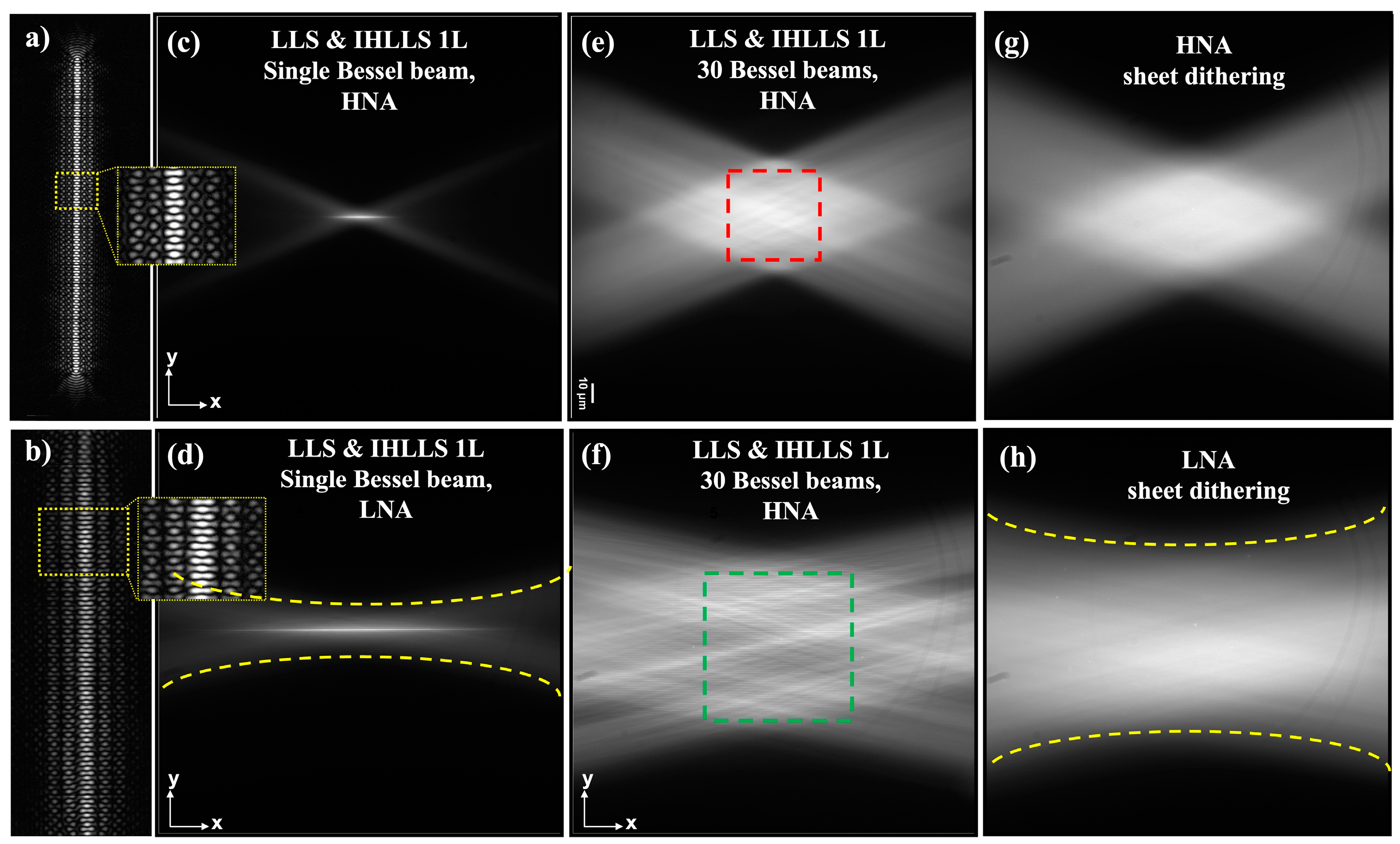
The beams generated by using the two annuli are shown in Figure 3. The upper row shows the optical lattice generated with the HNA annulus and the bottom row the optical lattice generated by the LNA annulus. Optical lattices can be designed to balance the confinement and the thickness by adjusting the spacing between each pair of beams. As an example, the lattice in Figure 3a is designed as a coherent superposition of 30 Bessel beams with a spacing of 0.99. Similarly, the lattice in Figure 3b is designed by using 26 Bessel beams with a spacing of 1.755. A single Bessel beam is shown in Figure 3c,d, respectively. We can see that the lower NA beam has a Gaussian-like shape. The beams at the sample plane, corresponding to the patterns in Figure 3a,b, are shown in Figure 3e,f, and the same beams but with the dithered mode are shown in Figure 3g,h.

3. Results

To examine the effects of applying IHLLS holography with LNA, we performed three experiments for this study.

3.1. LLS and IHLLS 1L Imaging with LNA

The first was done using the conventional LLS pathway where the z-galvo was stepped in $\delta z=0.101\mathsf{\mu }\mathrm{m}$ increments through the focal plane of a 25× Nikon objective, for a displacement of $\mathsf{\Delta }z=40\mathsf{\mu }\mathrm{m}$, Figure 4a. The detection objective was simultaneously moved the same distance with a z-piezo controller. The second set of images was obtained using the IHLLS 1L with a focal length f_SLM= 400 mm displayed on the SLM, where both the z-galvo and z-piezo were again stepped with the same $\delta z=0.101\mathsf{\mu }\mathrm{m}$ increments through the focal plane of the objective for the same displacement $\mathsf{\Delta }z=40\mathsf{\mu }\mathrm{m}$, Figure 4b. The scanning area in a conventional LLS with HNA is at best 52 × 52 μm² or 78 × 78 μm² in a conventional LLS with LNA (green dashed rectangles). Therefore, to enlarge the scanned region these ROI areas can be moved in a mosaic fashion by moving the sample.

3.2. IHLLS 2L Imaging

Our incoherent system enables full complex-amplitude modulation of the emitted light for extended FOV and depth. The second set of images was obtained using the IHLLS pathway with two super-imposed diffractive lenses displayed on the SLM comprising randomly selected pixels (IHLLS 2L), where only the z-galvo was moved within the same $\mathsf{\Delta }z=40\mathsf{\mu }\mathrm{m}$ displacement range, above and below the reference focus position of the objective (which corresponds to the middle of the camera FOV), at z_galvo = ±40 μm, ±30 μm, ±20 μm, ±10 μm, and 0 μm, Figure 5. The two wavefronts interfere with each other at the camera plane, to create Fresnel holograms. Four interference patterns were created using a phase shifting technique (θ = 0, θ = π/2, θ = π, θ = 3π/2) and further combined mathematically to obtain the complex amplitude of the object point at the camera plane.

The max projection of all z-planes where the beads were found are displayed in Figure 6a. They show the complex holograms propagated to the best focal plane. We observed that IHLLS 2L performed better in comparison to the conventional LLS system in dithering mode regarding the scanning/detection area. The scanned area with detected beads in an IHLLS 2L system with LNA is the full FOV of the CMOS detector while the scanned area with detected beads in a LLS system with LNA is about 78 × 78 μm². In terms of axial resolution, we already showed [9] that the axial resolution of IHLLS 2L was higher than that of LLS because the objects are localized with greater precision using diffraction software packages.

4. Conclusions

The approach of using lower-NA (LNA) masks to generate lattice light sheets forms beams that approximate Gaussian rather than Bessel beams. This provides a tradeoff between the size of the imaged beam and the resolution of the ultimate image in the z-plane. This has advantages for imaging objects at larger intercellular scales. Here, we demonstrate that even with these longer but lower-resolution beams, the IHLLS approach to generate holograms to resolve 3D positional information is functional. In fields of study such as neuroscience, where the cell structure is complex but at large scales, this approach will enable the resolution of complex 3D structures capturing structures as large as 200 µm in length.

References

1. Huisken, J.; Swoger, J.; Del Bene, F.; Wittbrodt, J.; Stelzer, E.H.K. Optical Sectioning Deep Inside Live Embryos by Selective Plane Illumination Microscopy. Science 2004, 305, 1007–1009. [Google Scholar] [CrossRef]
2. Davidovits, P.; Egger, M.D. Scanning Laser Microscope. Nature 1969, 223, 831. [Google Scholar] [CrossRef] [PubMed]
3. Pampaloni, F.; Ansari, N.; Girard, P.; Stelzer, E.H.K. Light sheet-based fluorescence microscopy (LSFM) reduces phototoxic effects and provides new means for the modern life sciences. In Proceedings of the Advanced Microscopy Techniques II, Munich, Germany, 22 May 2011; p. 80860Y. [Google Scholar]
4. Laissue, P.P.; Alghamdi, R.A.; Tomancak, P.; Reynaud, E.G.; Shroff, H. Assessing phototoxicity in live fluorescence imaging. Nat. Methods 2017, 14, 657–661. [Google Scholar] [CrossRef] [PubMed]
5. Stelzer, E.H.K.; Strobl, F.; Chang, B.-J.; Preusser, F.; Preibisch, S.; McDole, K.; Fiolka, R. Light sheet fluorescence microscopy. Nat. Rev. Methods Prim. 2021, 1, 73. [Google Scholar] [CrossRef]
6. Gao, L.; Shao, L.; Chen, B.-C.; Betzig, E. 3D live fluorescence imaging of cellular dynamics using Bessel beam plane illumination microscopy. Nat. Protoc. 2014, 9, 1083–1101. [Google Scholar] [CrossRef] [PubMed]
7. Gao, L. Optimization of the excitation light sheet in selective plane illumination microscopy. Biomed. Opt. Express 2015, 6, 881–890. [Google Scholar] [CrossRef] [PubMed]
8. Chen, B.-C.; Legant, W.R.; Wang, K.; Shao, L.; Milkie, D.E.; Davidson, M.W.; Janetopoulos, C.; Wu, X.S.; Hammer, J.A.; Liu, Z.; et al. Lattice light-sheet microscopy: Imaging molecules to embryos at high spatiotemporal resolution. Science 2014, 346, 1257998. [Google Scholar] [CrossRef] [PubMed]
9. Potcoava, M.; Mann, C.; Art, J.; Alford, S. Spatio-temporal performance in an incoherent holography lattice light-sheet microscope (IHLLS). Opt. Express 2021, 29, 23888–23901. [Google Scholar] [CrossRef] [PubMed]
Figure 1. (a) The LLS instrument [8]; (b) the diffraction annular mask filters of inner diameter, NAin, and outer diameter, NAout, to filter out undiffracted light and unwanted higher diffraction orders; (c) the detection arms for the LLS instrument with the IHLLS detection arm incorporated; and (d) optical schematics of IHLLS. The LLS and IHLLS with HNA use higher NAout and a shorter light sheet (more like Bessel beams), here NAout = 0.55, NAin = 0.48, and sheet length 15 μm. The LLS and IHLLS with LNA use lower NAout and longer light sheet (more like Gaussian beams), here NAout = 0.3, NAin = 0.275, and sheet length 75 μm. The detection magnification Mdet = 62.5 and the illumination wavelength λ e x c i t a t i o n n = 488 nm. The LLS, or IHLLS 1L with one diffractive lens, fSLM = 400 mm, are used for calibration purposes. The IHLLS 2L with two diffractive lenses, fd1 = 220 mm and fd2 = 2356 mm, are used for incoherent imaging. Lenses L1=L4 with focal lengths 175 mm, L2=L3 with focal lengths 100 mm; mirrors M1, M2, M3; fp1 and fp2 are the imaging positions of the two diffractive lenses, fd1 and fd2.
Engproc 34 00016 g001
Figure 2. Excitation and scanning geometry in LLS, IHLLS Systems. (a) The diffraction mask is conjugated with the BFP of the excitation objective; (b) the scanning geometry in LLS and IHLLS 1L, the z−galvo and z−piezo are moved along the z axis to acquire imaging stacks; (c) The scanning geometry in IHLLS 2L; the z-galvo is moved at various z positions but the z-piezo is kept fixed; (d) The FOV in a conventional LLS system or the incoherent version with one diffractive lens, with dithering scanning modality and HNA, is about 52 × 52 μm2 (red area); (e) the diffractive lens effect in IHLLS 2L system. Excitation objective: Special Optics 0.65 NA, 3.74 mm working water dipping lens; detection objective: Nikon CFI Apo LWD 25×—water dipping, 1.1 NA, 3 mm working distance.
Engproc 34 00016 g002
Figure 3. Optical lattice generation using HNA and LNA annuli; (a) HNA, 30 Bessel beams optical lattice with 0.99 spacing; the width of the light sheet in the center of the FOV is about 400 nm; (b) LNA, 26 Bessel beams optical lattice with 1.755 spacing; the width of the light sheet in the center of the FOV is about 800 nm; (c,d) Single Bessel beam at the sample plane; and (e,f) the Bessel beams corresponding to the optical lattices from (a,b) at the sample plane. The scanning area in a conventional LLS (HNA) is at best 52 × 52 μm2 (red square in (e)), and in a conventional LLS (LNA) about 78 × 78 μm2 (green square in (f)); (g,h) The Bessel beams corresponding to the optical lattices from (a,b) with the dithered mode at the sample plane.
Engproc 34 00016 g003
Figure 4. Tomographic imaging of 0.5 µm polystyrene beads, maximum FOV 208 × 208 µm2, in a conventional LLS (a) and IHLLS 1L of focal length 400 nm (b), without deconvolution, with LNA. On the sides and above are shown the max projections through the volume (400 z-galvo steps). The Bessel beams are displayed in the upper left corner of each xy-projection to show the orientation of the beams, FOV 208 × 208 µm2. The area enclosed inside the colored dashed rectangles, in the corner insets of (a,b), are as follows: green—the scanning area for the original LLS with LNA, 78 × 78 µm2, and yellow—the maximum FOV scanning area for the IHLLS 2L. We notice that LLS and IHLLS 1L cannot achieve the maximum FOV. The maximum FOV is achieved by using the IHLLS 2L, as showing in the next section.
Engproc 34 00016 g004
Figure 5. IHLLS 2L 500 nm beads holography, intensity images at phase shift, θ = 0; z-galvo position: (a) 40 μm, (b) 30 μm, (c) 20 μm, (d) 10 μm, (e) 0 μm, (f) −40 μm, (g) −30 μm, (h) −20 μm, and (i) −10 μm.
Engproc 34 00016 g005
Figure 6. Volume imaging comparison between the IHLLS 2L and LLS with LNA; (a) IHLLS 2L bead volume reconstruction; (b) LLS bead volume imaging. The green rectangle in the middle of the image represents the scanning area of the conventional LLS system in the dithering mode.
Engproc 34 00016 g006
Disclaimer/Publisher’s Note: The statements, opinions and data contained in all publications are solely those of the individual author(s) and contributor(s) and not of MDPI and/or the editor(s). MDPI and/or the editor(s) disclaim responsibility for any injury to people or property resulting from any ideas, methods, instructions or products referred to in the content.