Abstract
Autonomous navigation is one of the key tasks in the development of control systems for real autonomous mobile objects. This paper presents the developed technology for accurately determining the position of a mobile robot in an autonomous operating mode without an external positioning system. The approach involves using a high-precision model of a real robot identified by a neural network. The robot adjusts its position, determined using odometry and video camera, according to the position of the robot, obtained using an accurate model. To train the neural network, a training set is used that takes into account the features of the movement of a wheeled robot, including wheel slip. In the experimental part, the problem of autonomous movement of a mobile robot along a given trajectory is considered.
1. Introduction
Currently, there are many types of navigation of autonomous unmanned robots. Satellite navigation is certainly a common way. However, it also has a number of applicability limitations. For example, indoors, the satellite signal usually does not reach devices through concrete and metal structures. In this case, due to the fact that the space inside buildings is often limited to relatively small areas, it is possible to use navigation tools such as triangulation [1], navigation through various markers such as QR codes [2,3], barcodes [4], ArUco markers for position correction [5,6,7], and SLAM navigation [8,9], as well as combinations of the above methods.
In unexplored spaces, the most promising of the mentioned technologies is the SLAM navigation method [10]. This method can be used in an unprepared and unknown to the robot room to create a map and then use it. At present, this concept is widely used in the field of robotics for solving problems of autonomous motion [11,12,13]. According to SLAM, the robot needs to know its location at every moment of time, and also gradually scans the surrounding space with the help of sensors, thus compiling a map of the area. The map is built gradually as the robot explores new areas.
The main source of information about the location of the robot is odometry obtained in one way or another (wheels, computer vision, IMU, or a combination of both). However, any sensory system has its weak points. Therefore, for example, cameras can fail when lighting changes, or wheel slip can occur, causing an odometry error. In this regard, it becomes necessary to support the navigation system in some way independent of the readings of the sensors. This explains the relevance of this study.
The paper proposes the use of model-based navigation as a parallel system. In this case, one system can correct its values relative to the other.
Receiving a mathematical model for the control object is often time-consuming and sometimes even impossible using traditional methods. To build a mathematical model of a robot, the laws of theoretical mechanics and the Lagrange equations of the second kind for generalized coordinates are used. It should be noted that the analytical derivation of the robot dynamics equations in most cases will not accurately determine some parameters of the model, for example, friction coefficients of the robot moving parts or moments of inertia of rotating structures. Thus, the analytical output of mechanics equations allows one to build models with accuracy to the values of some parameters.
In view of the increasing diversity and extremely complex nature of control objects, including the variety of modern robotic systems, the identification problem is becoming increasingly important, which allows one to build a mathematical model of the control object, having input and output data about the system. Conducting experiments in order to identify the correspondence of the mathematical model to a real object is the necessary stage of solving the identification problem.
The identification of a nonlinear system is of particular interest, since most real systems have nonlinear dynamics, and if, earlier, the identification of a system model consisted of the selection of optimal parameters for the selected structure, then the emergence of modern machine learning methods opens up broader prospects and allows one to automate the identification process itself. Thus, this process should also be automated and, therefore, must be considered as the task for machine learning.
A modern technique to identify a mathematical model of a robot is the use of artificial neural networks. To perform this, it is necessary, depending on the assumed complexity of the robot model, to choose the structure and type of the neural network, then, depending on the problem to be solved, select a set of controls and build a training sample. Next, it is necessary to train the neural network so that the resulting neural network reacts to control actions in the same way as a real object. It is this approach that is presented in this paper and applied in the described experiments for a mobile robot.
Further, the paper presents a mathematical formulation of the model identification problem. A universal approach for solving it based on modern methods of machine learning using neural networks is proposed. As an example, a solution to the navigation problem for a mobile wheeled robot based on the proposed approach using its identified model is presented.
2. Problem Statement of the Control Object Identification by an Artificial Neural Network
In the identification problem, the mathematical model of the control object is not fully or partially known, but the researcher has a real control object or its physical simulator. In this case, the real control object or physical simulator layout is an unknown function. The space of the input vectors of this function is the space of admissible controls for this object.
Let some control functions be set as functions of time
where , , is a compact set that takes into account control constraints, and is a limit value of time.
The control functions , , should be selected so that it is possible to determine dynamic abilities and speed limits in straight lines and at turns by the movement of the control object.
To obtain a training sample, it is necessary to conduct natural experiments. In the experiment, the control object is subjected to a given control , and at fixed times, , the state of the control object is stored, , , where is a number of time intervals for experiment with control , .
A training sample for an artificial neural network is a set of stored values of the vectors of the control and the state in determined moments of time.
The input vector for the artificial neural network is an element of the training sample , , .
The output vector for the artificial neural network must coincide with the state space vector for the next moment of time , , :
where is a function described by the artificial neural network.
A target functional of optimization in the machine learning process of the artificial neural network is
In this case, the trained neural network is an approximation of the mathematical model of the control object in the form of a system of finite-difference recurrent equations.
If the time interval was selected to be quite small, then it is possible to use the artificial neural network as approximation of right parts of ordinary differential equation system in the Cauchy form. For this purpose, it is necessary to determine a rate of change of state variables for each time moment:
If the rate vector (5) is used as the output vector when training the neural network, then the mathematical model of the control object has the following form:
An important step in system identification is to determine the type of model used, since the overwhelming majority of methods implement the so-called parametric identification [14]. First, a certain model structure is selected, which is considered suitable for describing a given object. Next, an identification experiment is carried out in which the input and output signals are measured, and then the identification method implements the tuning of the model parameters in accordance with some adaptive laws, so that the response of the model to the input signal can approximately correspond to the response of the real system to the same input action. Most often, object identification is used using linear systems [15], since it is easy to determine the effect of various input signals on the output for them. Although linear models are attractive for many reasons, they have their limitations, especially since all physical systems are nonlinear to some extent, and in many cases linear models are not suitable for representing these systems. In this regard, there is currently a significant interest in methods for identifying nonlinear systems, especially using machine learning methods based on neural networks [16,17,18].
Neural networks, being a universal approximator, provide a powerful tool for identifying nonlinear systems. In view of the wide distribution and availability of software, neural networks have gained immense popularity. Combined approaches have also been developed, based, for example, on the reference model [19]. This article presents the implementation of a combined approach to the identification of a control object based on a neural network [20].
3. Application Object Description
A wheeled mobile robot shown in Figure 1 is taken as a control object.
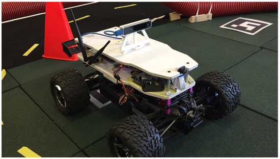
Figure 1.
A control object.
The work uses a mixed approach to identification, when part of the object model is known based on physical laws, and the other part is determined by a neural network trained on the basis of a specially formed training sample.
The robot motion model is described by a system of differential equations:
where define the object state, and are control signals.
Robot control is implemented using two signals: the desired linear velocity and the desired angular velocity . In the model (7), it is assumed that control signals are completely directly transmitted to the system , . In fact, a completely different picture is observed: firstly, the speeds cannot change infinitely quickly, and the system always has a certain dynamics, and secondly, as a rule, there is some regulator at a lower level that directly controls the voltage supplied to the motors. Therefore, in order to adequately describe the robot motion model, we introduced two additional equations into the (7) system that describe an object’s dynamics.
where and are unknown functions to be identified.
Factors such as friction of the wheels on the surface, inertia, and uneven distribution of the robot’s mass do not allow writing the functions in an explicit form.
For the numerical implementation of the identification problem, Equation (8) is presented in the finite-difference form with the time step :
To identify the system, we used the approximation of the function F by the parametric function . The learning function with parameters takes the current state of the robot, the control vector, and the time step as input, and outputs the state of the robot at the next moment of time:
4. ANN Model Identification
For training, the principle of supervised learning was chosen, in which the neural network is trained using the training dataset “input–reference output”, and then checked using a set of validation and test data that did not fall into the training sample.
To collect data, multiple runs of the robot were implemented under various types of control. Figure 2 and Figure 3 show the example trajectories and sample control data.
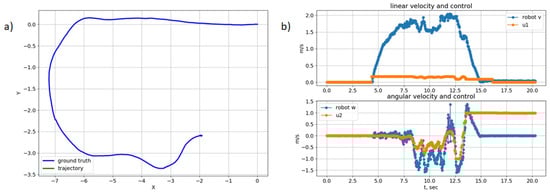
Figure 2.
Sample 1: (a) trajectory; (b) control.
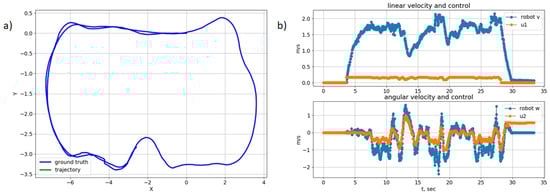
Figure 3.
Sample 2: (a) trajectory; (b) control.
An artificial neural network with the multilayer perceptron architecture was chosen as the training model (10). PyTorch was used to train the neural network. A neural network with three layers was chosen, with 128 neurons on all hidden layers, an RELU activation function, and Adam optimization algorithm.
To assess the quality of the model, the accuracy of predicting the trajectory of movement by the model was evaluated on passages that were not included in the training sample. The neural network receives as input the initial state of the system and the control sequence for the test drive. As in the training phase, the trajectory of the robot’s movement is predicted. To compare the predicted and actual trajectories, the metric was used—the absolute translation error:
where N is the number of points in the trajectory; and are actual trajectory point coordinates; and are coordinates of the predicted trajectory point.
To assess the quality of the predicted angle, the (mean absolute error) metric was used.
where is the actual value of the yaw angle, and is the predicted value of the yaw angle.
The results of simulations of the trained neural network model are shown in Figure 4 and Figure 5. As can be seen from the presented plots, the robot copes with the task of following the given trajectory even in the complex environment with strong surface slopes.
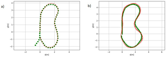
Figure 4.
The trajectory to follow is given by green points at the distance of (a) 30 cm; (b) 20 cm. The robots’s trajectory is a red line.
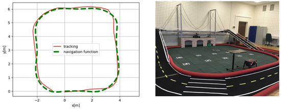
Figure 5.
The robot’s trajectory (red line) in a complex environment of the Robotic Center of FRC CSC RAS.
5. Discussion
This paper presents an approach to the localization of a mobile robot based on the identified neural network model. The presented results show how the robot copes quite accurately with the task of following various trajectories. The resulting neural network model can be used as an independent method of localization or as an auxiliary algorithm for correcting the position in case of failure of sensors and cameras.
Author Contributions
Conceptualization, I.P. and E.S.; methodology, A.D. and E.S.; software, I.P.; validation, E.S.; formal analysis, A.D.; investigation, I.P. and E.S.; data curation, E.S.; writing—original draft preparation, E.S.; writing—review and editing, E.S. All authors have read and agreed to the published version of the manuscript.
Funding
This research received no external funding.
Institutional Review Board Statement
Not applicable.
Informed Consent Statement
Not applicable.
Data Availability Statement
Not applicable.
Conflicts of Interest
The authors declare no conflict of interest.
References
- Sharp, N.; Soliman, Y.; Crane, K. Navigating intrinsic triangulations. ACM Trans. Graph. 2021, 38, 55. [Google Scholar] [CrossRef]
- Li, Z.; Huang, J. Study on the use of Q-R codes as landmarks for indoor positioning: Preliminary results. In Proceedings of the 2018 IEEE/ION Position, Location and Navigation Symposium (PLANS), Monterey, CA, USA, 23–26 April 2018; pp. 1270–1276. [Google Scholar] [CrossRef]
- Novoselov, S.; Sychova, O.; Tesliuk, S. Development of the Method Local Navigation of Mobile Robot a Based on the Tags with QR Code and Wireless Sensor Network. In Proceedings of the 2019 IEEE XVth International Conference on the Perspective Technologies and Methods in MEMS Design (MEMSTECH), Polyana, Ukraine, 22–26 May 2019; pp. 46–51. [Google Scholar] [CrossRef]
- Zhou, C.; Liu, X. The Study of Applying the AGV Navigation System Based on Two Dimensional Bar Code. In Proceedings of the 2016 International Conference on Industrial Informatics—Computing Technology, Industrial Information Integration (ICIICII), Intelligent Technology, Wuhan, China, 3–4 December 2016; pp. 206–209. [CrossRef]
- Sani, M.F.; Karimian, G. Automatic navigation and landing of an indoor AR drone quadrotor using ArUco marker and inertial sensors. In Proceedings of the 2017 International Conference on Computer and Drone Applications (IConDA), Kuching, Malaysia, 9–11 November 2017; pp. 102–107. [Google Scholar] [CrossRef]
- Marut, A.; Wojtowicz, K.; Falkowski, K. ArUco markers pose estimation in UAV landing aid system. In Proceedings of the 2019 IEEE 5th International Workshop on Metrology for AeroSpace (MetroAeroSpace), Turin, Italy, 19–21 June 2019; pp. 261–266. [Google Scholar] [CrossRef]
- Tian, W.; Chen, D.; Yang, Z.; Yin, H. The application of navigation technology for the medical assistive devices based on Aruco recognition technology. In Proceedings of the 2020 IEEE/RSJ International Conference on Intelligent Robots and Systems (IROS), Las Vegas, NV, USA, 24 October 2020–24 January 2021; pp. 2894–2899. [Google Scholar] [CrossRef]
- Geng, K.; Chulin, N.A. UAV Navigation Algorithm Based on Improved Algorithm of Simultaneous Localization and Mapping with Adaptive Local Range of Observations. Her. Bauman Mosc. State Tech. Univ. Ser. Nat. Sci. 2017, 3, 114. [Google Scholar] [CrossRef]
- Won, D.H.; Chun, S.; Sung, S.; Kang, T.; Lee, Y.J. Improving mobile robot navigation performance using vision based SLAM and distributed filters. In Proceedings of the 2008 International Conference on Control, Automation and Systems, Seoul, Republic of Korea, 14–17 October 2008; pp. 186–191. [Google Scholar] [CrossRef]
- Cheeseman, P.; Smith, R.; Self, M. A stochastic map for uncertain spatial relationships. In Proceedings of the 4th International Symposium on Robotics Research, Santa Cruz, CA, USA, 9–14 August 1987; pp. 467–474. [Google Scholar]
- Lu, F.; Milios, E. Globally Consistent Range Scan Alignment for Environment Mapping. Auton. Robot. 1997, 4, 333–349. [Google Scholar] [CrossRef]
- Biswas, J.; Veloso, M. Depth camera based indoor mobile robot localization and navigation. In Proceedings of the IEEE International Conference on Robotics and Automation, St. Paul, MN, USA, 14–18 May 2012; pp. 1697–1702. [Google Scholar] [CrossRef]
- Tu, Y.; Huang, Z.; Zhang, X.; Yu, W.; Xu, Y.; Chen, B. The Mobile Robot SLAM Based on Depth and Visual Sensing in Structured Environment. In Robot Intelligence Technology and Applications 3; Kim, J.H., Yang, W., Jo, J., Sincak, P., Myung, H., Eds.; Advances in Intelligent Systems and Computing Series; Springer: Cham, Switzerland, 2015; Volume 345. [Google Scholar]
- Zeng, R.; Kang, Y.; Yang, J.; Zhang, W.; Wu, Q. Terrain Parameters Identification of Kinematic and Dynamic Models for a Tracked Mobile Robot. In Proceedings of the 2018 2nd IEEE Advanced Information Management, Communicates Electronic and Automation Control Conference (IMCEC), Xi’an, China, 25–27 May 2018; pp. 575–582. [Google Scholar] [CrossRef]
- Cox, P.; Toth, R. Linear parameter-varying subspace identification: A unified framework. Automatica 2021, 123, 109296. [Google Scholar] [CrossRef]
- De León, C.L.; Vergara-Limón, S.; Vargas-Treviño, M.A.; López-Gómez, J.; Gonzalez-Calleros, J.M.; González-Arriaga, D.M.; Vargas-Treviño, M. Parameter Identification of a Robot Arm Manipulator Based on a Convolutional Neural Network. IEEE Access 2022, 10, 55002–55019. [Google Scholar] [CrossRef]
- Ge, W.; Wang, B.; Mu, H. Dynamic Parameter Identification for Reconfigurable Robot Using Adaline Neural Network. In Proceedings of the 2019 IEEE International Conference on Mechatronics and Automation (ICMA), Tianjin, China, 4–7 August 2019; pp. 319–324. [Google Scholar] [CrossRef]
- Liu, G.P. Nonlinear Identification and Control: A Neural Network Approach; Springer Science & Business Media: Berlin/Heidelberg, Germany, 2012. [Google Scholar]
- Williams, G.; Drews, P.; Goldfain, B.; Rehg, J.M.; Theodorou, E.A. Aggressive driving with model predictive path integral control. In Proceedings of the 2016 IEEE International Conference on Robotics and Automation (ICRA), Stockholm, Sweden, 16–21 May 2016; pp. 1433–1440. [Google Scholar]
- Shmalko, E.; Rumyantsev, Y.; Baynazarov, R.; Yamshanov, K. Identification of Neural Network Model of Robot to Solve the Optimal Control Problem. Inform. Autom. 2021, 20, 1254–1278. [Google Scholar] [CrossRef]


Disclaimer/Publisher’s Note: The statements, opinions and data contained in all publications are solely those of the individual author(s) and contributor(s) and not of MDPI and/or the editor(s). MDPI and/or the editor(s) disclaim responsibility for any injury to people or property resulting from any ideas, methods, instructions or products referred to in the content. |
© 2023 by the authors. Licensee MDPI, Basel, Switzerland. This article is an open access article distributed under the terms and conditions of the Creative Commons Attribution (CC BY) license (https://creativecommons.org/licenses/by/4.0/).