Additional Requirement in the Formulation of the Optimal Control Problem for Applied Technical Systems ^†

Abstract

This paper considers the difficulties that arise in the implementation of solutions to the optimal control problem. When implemented in real systems, as a rule, the object is subject to some perturbations, and the control obtained as a function of time as a result of solving the optimal control problem does not take into account these factors, which leads to a significant change in the trajectory and deviation of the object from the terminal goal. This paper proposes to supplement the formulation of the optimal control problem. Additional requirements are introduced for the optimal trajectory. The fulfillment of these requirements ensures that the trajectory remains close to the optimal one under perturbations and reaches the vicinity of the terminal state. To solve the problem, it is proposed to use numerical methods of machine learning based on symbolic regression. A computational experiment is presented in which the solutions of the optimal control problem in the classical formulation and with the introduced additional requirement are compared.

1. Introduction

The main disadvantage of the optimal control problem [1] is that its solution is an optimal control as a function of time, and it cannot be implemented in practice since its implementation leads to an open control system that is insensitive to model disturbances.

Consider a well-known optimal control problem

$$\begin{array}{ccc}\hfill {\dot{x}}_1& =& x_2,\hfill \\ \hfill {\dot{x}}_2& =& u,\hfill \end{array}$$

(1)

where $\mathbf{x}={[x_1 x_2]}^T$ is a state vector, u is a control signal.

The control values are limited

$$-1\le u\le 1.$$

(2)

It is necessary to find a control that will move the object (1) from the initial state

$$\mathbf{x}\left(0\right)={[1 1]}^T,$$

(3)

to the given terminal position

$${\mathbf{x}}^f={[0 0]}^T$$

(4)

as fast as possible

$$J=t_f\to \min .$$

(5)

The analytical solution of the stated problem was presented in [1]. According to the maximum principle, the optimal control takes only limit values (2) and has no more than one switch. According to (3), initially, the control has the value $u=-1$. Then, when a certain state is reached, the control switches to the value $u=1$.

$$u=\left\{\begin{array}{c}-1,\mathrm{if}t<t^{\ast }\hfill \\ 1,\mathrm{otherwise}\hfill \end{array}\right.$$

(6)

where $t^{\ast }$ is the moment of control switching.

Let us find the moment of switching. A particular solution of the system (1) from the initial state (3) has the following form

$$\begin{array}{ccc}\hfill x_1& =& -0.5t^2+t+1,\hfill \\ \hfill x_2& =& -t+1.\hfill \end{array}$$

(7)

The general solution (1) for the control $u=+1$ is the following

$$\begin{array}{ccc}\hfill x_1& =& 0.5t^2+x_{2,0}t+x_{1,0},\hfill \\ \hfill x_2& =& t+x_{2,0},\hfill \end{array}$$

(8)

where $x_{1,0}$, $x_{2,0}$ are the coordinates of the switching point.

Let us express in (8) $x_1$ as a function of $x_2$

$$x_1=x_2^2-0.5x_{2,0}^2+x_{1,0},$$

(9)

The relation for the switching point follows from the terminal conditions (4)

$$x_{1,0}=0.5x_{2,0}^2.$$

(10)

Let us now find the moment of time for a particular solution (7) that satisfies the relation (10).

$$\begin{array}{ccc}\hfill -0.5t^2+t+1& =& 0.5{(-t+1)}^2;\hfill \\ \hfill t^2-2t-0.5& =& 0;\hfill \\ \hfill t^{\ast }=1+\sqrt{1.5}& =& 2.22474487.\hfill \end{array}$$

(11)

The switching time (11) is the solution to this optimal control problem. To determine the value of the functional (5), we calculate the coordinates of the switching point. Substituting (11) into the particular solution (7), we obtain

$$x_1=-0.75, x_2=\sqrt{1.5}.$$

(12)

From the second equation in (8), we obtain the optimal time of reaching the terminal state

$$\tilde{t}=t^{\ast }+\sqrt{1.5}=3.44948974.$$

(13)

Now, we introduce perturbations into the initial conditions (3)

$$x_1\left(0\right)=1+{\delta }_1, x_2\left(0\right)=1+{\delta }_2,$$

(14)

where ${\delta }_1$, ${\delta }_2$ are random variables from a limited range.

During the time $t^{\ast }$, the object does not get to the switching point (12), and after switching accordingly, does not get into the terminal state. Based on the optimal value of the functional (13), let us limit the control time to $t^{+}=3.5$ and determine the state of the object at the moment $t^{+}$, taking into account the switching of the control at the moment (11)

$$\begin{array}{ccc}\hfill {\widehat{x}}_{1,0}& =& -0.5{t^{\ast }}^2+(1+{\delta }_2)t^{\ast }+1+{\delta }_1,\hfill \\ \hfill {\widehat{x}}_{2,0}& =& -t^{\ast }+1+{\delta }_2,\hfill \\ \hfill x_1\left(t^{+}\right)& =& 0.5{(t^{+}+t^{\ast })}^2+{\widehat{x}}_{2,0}(t^{+}-t^{\ast })+{\widehat{x}}_{1,0}=\hfill \\ \hfill & & 0.00127565-(1.27525513+t^{\ast }){\delta }_2+{\delta }_1,\hfill \\ \hfill x_2\left(t^{+}\right)& =& t^{+}-t^{\ast }+{\widehat{x}}_{2,0}=0.05051026+{\delta }_2.\hfill \end{array}$$

(15)

Figure 1 shows trajectories of eight randomly perturbed solutions of the problem (1)–(5) from the range

$$x_1\left(0\right)=1\pm 0.25, x_2\left(0\right)=1\pm 0.25.$$

(16)

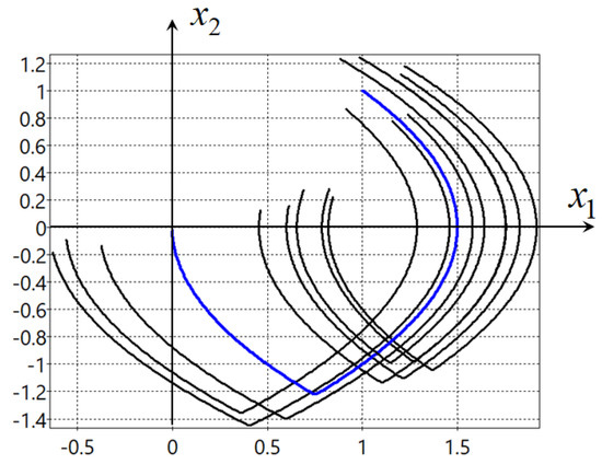
Figure 1. Optimal and perturbed solutions with control (6).

In Figure 1, the blue curve represents the optimal unperturbed solution.

All perturbed solutions do not reach the terminal state. It is obvious from the plots that the solution of the optimal control problem as a function of time (6) cannot be implemented in practice since according to the model (1) with control (6) due to disturbances, it is impossible to assess the state of the control object.

In this regard, it is necessary to introduce additional requirements into the formulation of the optimal control problem so that the resulting controls can be directly implemented on a real plant.

2. Optimal Control Problem Statement with Additional Requirement

Consider the formulation of the optimal control problem, the solution of which can be directly implemented on the plant.

Given the mathematical model of the control object

$$\dot{\mathbf{x}}=\mathbf{f}(\mathbf{x},\mathbf{u}),$$

(17)

where $\mathbf{x}\in {\mathbb{R}}^n$, $\mathbf{u}\in \mathrm{U}\subseteq {\mathbb{R}}^m$, $\mathbf{f}={[f_1(\mathbf{x},\mathbf{u})\dots f_n(\mathbf{x},\mathbf{u})]}^T$.

Given the initial

$$\mathbf{x}\left(0\right)={\mathbf{x}}^0\in {\mathbb{R}}^n.$$

(18)

and terminal conditions

$$\mathbf{x}\left(t_f\right)={\mathbf{x}}^f\in {\mathbb{R}}^n,$$

(19)

where $t_f$ is the time to reach the terminal conditions, not specified, but limited, $t_f\le t^{+}$, $t^{+}$ is the specified limit time of the control process.

A quality criterion is set. It may include conditions for fulfilling phase constraints

$$J_1=\underset{0}{\overset{t_f}{\int }}{f}_0(\mathbf{u},\mathbf{x})dt\to \underset{\mathbf{u}\in \mathrm{U}}{min}.$$

(20)

We need to find a control in the form

$$\mathbf{u}=\mathbf{g}(\mathbf{x},t)\in \mathrm{U}.$$

(21)

The found control must be such that the particular solution $\mathbf{x}(t,{\mathbf{x}}^0)$ of the system

$$\dot{\mathbf{x}}=\mathbf{f}(\mathbf{x},\mathbf{g}(\mathbf{x},t))$$

(22)

from the initial state (18) reaches the terminal state (19) with the optimal value of the quality criterion (20). Moreover, the optimal particular solution $\mathbf{x}(t,{\mathbf{x}}^0)$ of the system (22) would have a neighborhood $\Delta \left(t\right)>0$ such that if for any other particular solution $\mathbf{x}(t,\mathbf{y})$ of the system (22) from another initial state $\mathbf{y}\in {\mathbb{R}}^n$ at time $t^{\prime }$, $0\le t^{\prime }\le t^{+}$

$$\parallel \mathbf{x}(t^{\prime },\mathbf{y})-\mathbf{x}(t^{\prime },{\mathbf{x}}^0)\parallel \le \Delta \left(t^{\prime }\right),$$

(23)

then $\forall t$, $t^{\prime }\le t\le t_f$, this particular solution does not leave the neighborhood of the optimal

$$\parallel \mathbf{x}(t,\mathbf{y})-\mathbf{x}(t,{\mathbf{x}}^0)\parallel \le \Delta \left(t\right), t^{\prime }\le t\le t_f.$$

(24)

The neighborhood $\Delta \left(t\right)$ shrinks near the terminal state. This means that for any particular solution from the neighborhood of the optimal one for which the conditions (23) are satisfied $\exists t^{″}<t^{+}$ such that

$$\parallel \mathbf{x}(t^{″},\mathbf{y})-\mathbf{x}(t^{″},{\mathbf{x}}^0)\parallel \le \epsilon ,$$

(25)

where $\epsilon$ is a given small positive value.

The existence of a neighborhood of the optimal solution in many cases can worsen the value of the functional. For example, in a problem with phase constraints, which are obstacles on the path of movement of the control object to the terminal state, the optimal trajectory often passes along the boundary of the obstacle. Such a trajectory will not have a neighborhood, so in this case, it is necessary to find another trajectory that will not be optimal according to the classical formulation of the optimal control problem but allows variations in the initial values with a small change in the value of the functional.

3. Overview of Methods for Solving the Extended Optimal Control Problem with Additional Requirement

Therefore, an additional requirement has been put forward in the formulation of the optimal control problem, which makes it possible to implement the obtained controls on real objects. Consider the existing methods for solving the problem in the presented extended formulation.

The solution to the problem of general control synthesis for a certain region of initial conditions leads to the fact that each particular solution from this region of initial conditions will be optimal. In this case, each particular solution has a neighborhood containing other optimal solutions. The neighborhood will be open, but will also shrink near the terminal state.

For the model (1), there is a solution to the problem of general control synthesis, in which a control is found that ensures the optimal achievement of the terminal state from any initial condition.

$$u^{\ast }=\left\{\begin{array}{c}-1,\mathrm{if}h(x_1,x_2)\ge 0\hfill \\ 1,\mathrm{otherwise}\hfill \end{array}\right.,$$

(26)

where

$$h(x_1,x_2)=\left\{\begin{array}{c}{x}_1+0.5x_2^2,\mathrm{if}{x}_1<0\hfill \\ x_1-0.5x_2^2,\mathrm{otherwise}\hfill \end{array}\right..$$

(27)

Plots of eight perturbed solutions for the object model (1) with control (26) are shown in Figure 2.

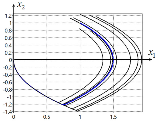
Figure 2. Optimal and perturbed solutions with control (26).

As can be seen from Figure 2, all perturbed solutions have reached the terminal state. This control (26) is practically feasible.

However, the problem of general control synthesis is a complex mathematical problem for which there is no universal numerical solution method. In this case, this problem was solved because the plant model is simple, the optimal control takes only two limit values, and for both of these values, general solutions of the differential equations of the model (1) are obtained.

Another approach to solving the optimal control problem and fulfilling additional requirements is stabilizing motion along the trajectory based on the theory of stability of A.M. Lyapunov [2]. As a result of constructing the stabilization system, the optimal trajectory should become asymptotically stable. The construction of such a stabilization system is not always possible; in particular, in the problem under consideration (1), the control resources are exhausted to obtain the optimal trajectory and there are no more control resources for the stabilization system.

Another approach that also allows solving the optimal control problem in the presented extended formulation with additional requirements is the synthesized control method. It consists of two stages [3,4]. Initially, the problem of control synthesis is solved in order to ensure the stability of the control object relative to some point in the state space. In the second stage, the problem of optimal control is solved, while the coordinates of the stability points of the control object are used as control. It should be noted that the solution of the control synthesis problem at the first stage will significantly change the mathematical model of the control object. When solving the control synthesis problem, the functional of the optimal control problem is not used to ensure stability; therefore, various methods for solving the control synthesis problem will lead to different mathematical models of a closed control system and to different solutions to the optimal control problem. The presence of a neighborhood with attraction properties for the optimal solution requires the choice of such a position of the stability points in the state space so that particular solutions from a certain region of initial states, being attracted to these stability points, are close to each other, moving to the terminal state.

Consider the application of the synthesized optimal control to problems (1)–(5). For stabilization system synthesis different methods can be used from traditional regulators [5] to modern machine learning techniques [6,7,8]. As far as the considered object is rather simple (1), it is enough to use a proportional regulator. Taking into account the limits on control, it has the following form

$$u=\left\{\begin{array}{c}\mathrm{sgn}\left(\tilde{u}\right),\mathrm{if}\left|\tilde{u}\right|>1\hfill \\ \tilde{u}--\mathrm{otherwise}\hfill \end{array}\right.,$$

(28)

where

$$\tilde{u}=k_1(x_1^{\ast }-x_1)+k_2(x_2^{\ast }-x_2).$$

(29)

The object is stable if $k_1>0$, $k_2>0$. A stable equilibrium point exists if $|\tilde{u}|<1$. The coordinates of the equilibrium point for the given $k_1$, $k_2$ depend on the values of $x_1^{\ast }$, $x_2^{\ast }$

$${\tilde{x}}_1=\frac{k_2{x}_2^{\ast }+k_1{x}_1^{\ast }}{k_1}, {\tilde{x}}_2=0.$$

(30)

As a result, we obtain the following control object model

$$\begin{array}{ccc}\hfill {\dot{x}}_1& =& x_2\hfill \\ \hfill {\dot{x}}_2& =& k_1(x_1^{\ast }-x_1)+k_2(x_2^{\ast }-x_2)\hfill \end{array}.$$

(31)

The control in the model is the vector ${\mathbf{x}}^{\ast }={[x_1^{\ast } x_2^{\ast }]}^T$, whose values are limited by the following inequalities

$$-1\le k_1(x_1^{\ast }-x_1)+k_2(x_2^{\ast }-x_2)\le 1.$$

(32)

To solve the problem of optimal control, we include in the quality criterion the accuracy of hitting the terminal state ${\mathbf{x}}^f={[0 0]}^T$

$$J_5=t_f+p_1\parallel {\mathbf{x}}^f-\mathbf{x}\parallel ,$$

(33)

where $t_f$ is a terminal time, $p_1$ is a weight coefficient, $p_1=1$.

When solving the problem, we divide the control time $t^{+}$ into intervals $\Delta t$, and on each interval, we look for the values $x_1^{\ast }$, $x_2^{\ast }$, taking into account the constraints (32). The following parameter values were used: $k_1=2$, $k_2=2$, $p_1=1$, $t^{+}=3.5$, ${\Delta }_t=0.5$, ${\epsilon }_1=0.001$. An evolutionary hybrid algorithm [9] was used for the solution. The optimal solution gave the value of the functional (33) $J_5=3.6343$.

Figure 3 shows particular solutions of the system (31) with random perturbations of the initial values in the range (16). The blue curve in the figure shows the unperturbed optimal solution. The black dots show the positions of the found ${\mathbf{x}}^{\ast }$ control points. As we see from the experimental results, the perturbed solutions stabilize in the vicinity of the optimal one. Compared to Figure 1, it is obvious that the resulting model (31) is feasible.

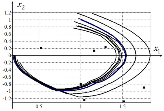
Figure 3. Perturbed and unperturbed solutions under synthesized optimal control.

4. Discussion

This paper raises the problem of the feasibility of optimal controls obtained as a result of solving the classical formulation of the optimal control problem. It is shown that when disturbances appear, the solutions turn out to be unsatisfactory. In the paper, an additional requirement for the desired control function is introduced. The introduced requirement ensures the stability of solutions near the optimal solution. Possible approaches to solving the proposed extended optimal control problem are considered. The best solution for problems (1)–(5) is the solution to the general control synthesis problem. However, for more complex objects, it is not always possible to solve the problem of general synthesis. This paper considers the method of synthesized optimal control, which satisfies the introduced requirement of the feasibility of optimal control, and at the same time finds solutions that are close to optimal through the use of machine learning methods and evolutionary algorithms.

References

- Pontryagin, L.S.; Boltyanskii, V.G.; Gamkreidze, R.V.; Mishchenko, E.F. The Mathematical Theory of Optimal Processes; Division of John Wiley and Sons, Inc.: New York, NY, USA, 1962. [Google Scholar]
- Krasovskii, N.N. Stability of Motion; Stanford University Press: Redwood City, CA, USA, 1963. [Google Scholar]
- Diveev, A.; Shmalko, E.; Serebrenny, V.; Zentay, P. Fundamentals of Synthesized Optimal Control. Mathematics 2021, 9, 21. [Google Scholar] [CrossRef]
- Shmalko, E. Feasibility of Synthesized Optimal Control Approach on Model of Robotic System with Uncertainties. In Electromechanics and Robotics; Ronzhin, A., Shishlakov, V., Eds.; Smart Innovation, Systems and Technologies; Springer: Singapore, 2022; Volume 232, pp. 131–143. [Google Scholar]
- Ang, K.H.; Chong, G.; Li, Y. PID control system analysis, design, and technology. IEEE Trans. Control Syst. Technol. 2005, 13, 559–576. [Google Scholar] [CrossRef]
- Hu, F.; Zeng, C.; Zhu, G.; Li, S. Adaptive Neural Network Stabilization Control of Underactuated Unmanned Surface Vessels With State Constraints. IEEE Access 2020, 8, 20931–20941. [Google Scholar] [CrossRef]
- Yu, H.; Park, S.; Bayen, A.; Moura, S.; Krstic, M. Reinforcement Learning Versus PDE Backstepping and PI Control for Congested Freeway Traffic. IEEE Trans. Control Syst. Technol. 2022, 30, 1595–1611. [Google Scholar] [CrossRef]
- Diveev, A.; Shmalko, E. Machine Learning Control by Symbolic Regression; Springer International Publishing: Cham, Switzerland, 2021. [Google Scholar]
- Diveev, A. Hybrid Evolutionary Algorithm for Optimal Control Problem. In Intelligent Systems and Applications; Arai, K., Ed.; Lecture Notes in Networks and Systems Series; Springer: Cham, Switzerland, 2023; Volume 544. [Google Scholar]
Disclaimer/Publisher’s Note: The statements, opinions and data contained in all publications are solely those of the individual author(s) and contributor(s) and not of MDPI and/or the editor(s). MDPI and/or the editor(s) disclaim responsibility for any injury to people or property resulting from any ideas, methods, instructions or products referred to in the content. |
© 2023 by the authors. Licensee MDPI, Basel, Switzerland. This article is an open access article distributed under the terms and conditions of the Creative Commons Attribution (CC BY) license (https://creativecommons.org/licenses/by/4.0/).