Abstract
The Leaf Area Index (LAI) is an important algorithm for studying the health status of vegetation. In this study, the impact of hydrocarbon micro-seepage on vegetation in Ugwueme was investigated using the LAI image classification approach. Landsat TM 1996, ETM+ 2006, and OLI 2016 satellite images that were acquired from the United States Geological Survey (USGS) portal were used to classify various LAI maps as low, moderate, and high classes. The spatial–temporal analysis revealed that the low, moderate, and high LAI density classification changed, respectively, from 41.24 km2 (50.43%), 33.98 km2 (41.54%), and 6.56 km2 (8.02%) in 1996 to 23.70 km2 (28.98%), 29.48 km2 (36.04%), and 28.60 km2 (34.97%) in 2006, and to 38.23 km2 (46.74%), 27.54 km2 (33.68%), and 16.01 km2 (19.58%) in 2016. The stimulation analysis shows that by 2030 (the 14-year planning period), the low, moderate, and high LAI density classifications will be 8.86 km2 (10.82%), 24.28 km2 (29.70%), and 48.63 km2 (59.46%), respectively. The study shows that LAI is an important algorithm that can be effectively used to study the health status of vegetation in an ecosystem.
1. Introduction
Hydrocarbon oil and gas located below the earth’s surface often accumulate in an impermeable underground reservoir. These oils and gases leak under high pressure and then outflow in a vertical or nearly vertical direction through weak geological structures, such as faults, joints, and discontinuities, to areas of low pressure before emerging on the earth’s surface as either macro- or micro-seepage [1,2]. Micro-seepages are invisible traces of light hydrocarbons that are detectable only by geochemical means [3,4]. During the vertical migration of oil and gas, oxidation–reduction reactions are established along migration paths, resulting in anomalies in surrounding sediments, soils, and vegetation [5,6]. Vegetation anomalies, mineralogical alterations, and the changes linked to electrical and magnetic fields often occur on or near the earth’s surface [7,8]. Among these anomalies and alterations, Shi et al. [9] reported that bleaching of red beds, enrichment of ferrous iron, clay minerals, and carbonate alterations, as well as vegetation anomalies, often express diagnostic spectral properties that can be studied with remote sensing technology [10]. Depending on climate, soil type, vegetation species, and location, micro-seepage has been found to have a tremendous impact on vegetation, yielding stress and eventually death [11,12].
Remote sensing (RS) is a fast, cheap, and non-destructive method that is used for interpreting anomalous zones [13]. It demonstrates the ability to detect changes in the spectral reflectance of vegetation [14]. Figure 1 depicts the spectral reflectance curve of vegetation. When electromagnetic energy interacts with vegetation, it is reflected, absorbed, or transmitted, depending on its chemical constituents or leaf structures [15]. When vegetation is stressed, the NIR bands are absorbed by the dead cells rather than reflected [16]. In the visible section, absorption is more pronounced at 0.45 µm and 0.66 µm. The absorptions within the blue and red regions respond strongly to the absorption of chlorophyll (chlorophyll-a and chlorophyll-b) bands. Healthy vegetation absorbs electromagnetic radiation in its visible region (0.4–0.7 µm). Near the 0.7 µm, red/infrared boundary, absorption decreases and reflection increases. From 0.7 to 1.3 µm, the reflectance is virtually constant before diminishing as the wavelengths get longer [16].
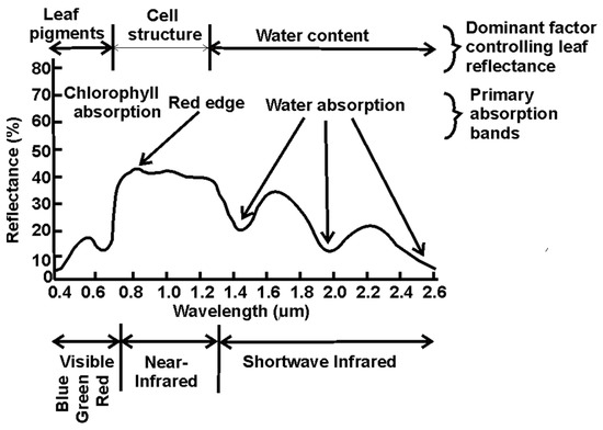
Figure 1.
Spectral Reflectance curve for vegetation [15].
Leaf Area Index (LAI), an important technique in remote sensing [17]. It is one of the robust vegetation indices that can be used to study the impact of hydrocarbon seepage on vegetation. Wang et al. [18] highlight that LAI is a vegetation structural index, defined as half the value of the overall green leaf area per its unit ground surface area. LAI has a lot of advantages. Some of these include the fact that they are employed in agricultural and ecological studies for a variety of objectives, such as yield evaluation, stress determination, and primary productivity, which are connected to photosynthesis, transpiration, respiration, and the carbon and nutrient cycles [19]. Thus, LAI is a crucial input for a variety of agricultural, ecological, climatic, and hydrological models, including models of canopy photosynthesis, crop growth, transpiration, precipitation, evaporation, and primary production. An important drawback of LAI is that it cannot be used to quantify stress on each plant species since different plants grow together as a community. LAI relates to the Soil Adjusted Vegetation Index (SAVI), and their relationship is depicted in equation 1 [19]. Due to the lack of soil, the SAVI minimizes the brightness reflection with the Normalized Difference Vegetation Index (NDVI). The NDVI is an indicator that explains the visible and near-infrared reflectance of vegetation that can be adopted to determine the density of greenness within an area of land [20]. The SAVI is calculated with equation 2 [21]. The study aims to stimulate the impact of hydrocarbon micro-seepage on forest ecosystems in Ugwueme from 1996 to 2030, based on the use of the Leaf Area Index algorithm and Markov chain model. Researchers such as Breda [22], Johckheere et al. [23], Weiss et al. [24] and Chen [25] had used experimental design, sample techniques, tools, and estimating theories for ground-based LAI measurements to monitor plant health. These methods for measuring LAI are often cumbersome and time-consuming. This study had used the time series LAI algorithm and Markov chain model for mapping and for stimulation analysis. Mapping and stimulating with RS tools is more rapid and has large coverage, as compared to the ground-based methods.
where NIR is the reflectance in the near infrared band, and red is the Red band [15].
LAI = −In [(0.69 − SAVI)/0.59]/0.91
2. Materials and Methods
2.1. Materials
In this study, Landsat 5 TM, 7 ETM+, and 8 OLI for 1996, 2006, and 2016 were used to model the LAI change dynamics. These Landsat images were all acquired through the United States Geological Survey portal (http://earthexplorer.usgs.gov/) on 6 January 1996 for Landsat 5TM, 12 January 2006 for Landsat 7, and 4 January 2016 for Landsat 8 OLI. All of the images were taken in the same season (dry season) and were cloud-free. They have a spatial resolution of 30 m and were chosen due to their quality and availability (Table 1).

Table 1.
Characteristics of the sensors used in the study.
2.2. Methods
Image Pre-Processing and Classification
Pre-processing is very critical in change detection analysis, as inaccuracies ascribed to image sensors, if not rectified, might result in erroneous results [26]. Pre-processing improves the quality of the image by eliminating radiometric and geometric flaws. In the study, image pre-processing, which included image gap-filling, sub-setting, enhancement, and radiometric corrections, was performed with the ArcGIS 10.5 and ERDAS Imagine 10.5 software packages. Zig-zag lines are present in all Landsat 7 ETM+ data acquired from the USGS after 31 May 2003. This error was the result of a failure in the ETM+ Scan Line Corrector. To rectify this line error in the ETM+ data, which were used for this study, radiometric correction was applied with the Landsat toolbox embedded in the ArcGIS 10.5 software. The World Geodetic System (WGS) 1984 ellipsoid was used to register satellite data with the Universal Transverse Mercator (UTM) zone 32N coordinate system. By integrating multiple satellite spectral bands in the RGB format for all the images used (1996, 2006, and 2016), the layer stacking tool of the ERDAS Imagine program was used to generate the Region of Interest (AOI) before overlaying the shape-file of the research area (Ugwueme) and then sub-setting. Image classification in remote sensing is classified as either supervised or unsupervised [7]. In this study, the supervised classification with the maximum likelihood classifier (MLC) approach was utilized for the classification process due to its ease of training [5]. In this process, clusters of images are defined as a class, and a class often occupies a section in the feature space. The training areas are created by digitizing each of the LAI classes, generated by band combinations, such as class 1 (low LAI), class 2 (moderate LAI), and class 3 (high LAI). The trend K is calculated as the degree of LAI class changes between the reference data (T2) and the initial data (T1) [27]. LAI classes that are reducing are shown with a negative sign (-), while those increasing are represented with a positive sign (+).
2.3. Stimulation of Future LAI Dynamics
2.3.1. Markov Chain Model
The Markov chain model (MCM) is a conditional model that represents the likelihood of a LAI type transiting from one mutually exclusive state (St) to another (St1) during a given time period [28]. Future LAI changes are frequently stimulated based on the transition probabilities of the previous or current LAI changes [29]. MCM often provides estimates of the spatial distribution of LAI changes as well as predictions of their magnitude and quantity. As shown in (3) and (4), the conditional probability equation defined by [30,31,32] for stimulation analysis is given as:
and
where pij is the transition probability matrix, n is the number of LAI types, and i and j, as well as St and St1, are the LAI statuses at time t and t1.
2.3.2. Cellular Automata Model
A cellular automata (CA) model is a discrete model for simulating complex activities in space and time [33]. It is a spatial dynamic system based on a transition rule that links the new state to the LAI type’s prior state. CA-based models can also depict non-linear and complicated, geographically distributed processes, providing insights into LAI change patterns at the local, national, regional, and global levels [34]. Cells, cell size, cell neighborhood, transition rules, and time are some of the model’s important components that must be taken into account for optimal stimulation results [35]. According to Subedi et al. [27] and Singh et al. [28], the CA model is expressed as follows in (5):
where S is the set of states of the finite cells, N is the number of neighboring cells, t and t + 1 are different times, and f is the transformation rule of local space.
2.3.3. CA–Markov Model
The CA–Markov model is a model that combines the theories of Markov and CA for future spatial–temporal analysis [22,36]. In remote sensing, the integrated CA–Markov model has advantages due to its simple calibration, effective efficiency with data, and capacity for complex patterns [37,38]. The CA–Markov model was applicable in this study for stimulation analysis.
3. Results and Interpretation
3.1. Classification Analysis and Rate of Changes
Table 2 shows the LAI classification and rate of change analysis. From the spatial–temporal analysis, we see that the category of moderate LAI classes decreased from 33.9750 km2 (41.54%) in 1996 to 29.4777 km2 (36.04%) in 2006 and to 27.5436 km2 (33.68%) in 2016. Throughout the study, the low and high LAI classes decreased and increased, respectively, from 41.2443 km2 (50.43%) and 6.5610 km2 (8.02%) in 1996, to 23.7006 km2 (28.98%) and 28.6020 km2 (34.97%) in 2006, and to 38.2266 km2 (46.74%) and 16.0101 km2 (19.58%) in 2016. Between 1996 and 2006, the low and moderate LAI classes experienced negative changes of −17.5437 km2 (−21.45%) and −4.4973 km2 (−5.5%), while the high LAI class experienced positive changes of 22.041 km2 (26.95%). From 2006 to 2016, the low LAI class accounted for a positive change of 14.526 km2 (17.76%), while the moderate and high LAI classes recorded negative changes of −1.9341 km2 (−2.36%) and −12.5919 km2 (−15.39%), respectively. The spatial–temporal analysis shows that vegetation changes are occurring in the study area. These changes are depicted with differences in the LAI classification maps and are the result of vegetation degradation due to the various degrees of impact and spread of the hydrocarbon seepage over the study years. The spread of hydrocarbon seepage in the year 2016 was higher than in 2006 and 1996; hence, the vegetation was more degraded in 2016 than in other study years. The higher the value of the vegetation index, the higher the likelihood that a substantial amount of green vegetation will cover the area. Lower LAI values indicate reduced or degraded vegetation. Figure 2 depicts LAI classification maps for the 1996, 2006, and 2016 study years. The maps were categorized into low, moderate, and high LAI classes. The yellow pixels depict areas of low LAI. The red and blue pixels show regions of moderate and high LAI. Low LAI areas have a low spread of hydrocarbon seepage, whereas moderate and high LAI areas have a moderate and high spread of hydrocarbon seepage, respectively.
Table 2.
The LAI density classification.
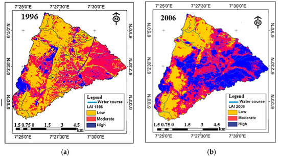
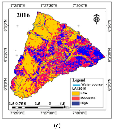
Figure 2.
LAI classification maps for (a) 1996, (b) 2006, and (c) 2016.
3.2. The Spectral Reflectance of Vegetation
Figure 3 depicts the differences in the spectral reflectance of solar energy between healthy and un-healthy (stressed) vegetation and within the visible and infrared sections of the electromagnetic spectrum. Here, the reflectance values of vegetation are plotted against the wavelength to show the degree of reflectance in the spectrum. Within the visible section of the spectrum, we see in Figure 3 that, from 1996 to 2016, healthy vegetation reflected more solar radiation than un-healthy (stressed) vegetation. However, the spectral reflectance curve of unhealthy (stressed) vegetation is affected owing to the decrease in efficiency of photosynthetic pigments, thereby yielding an increase in the reflectance values within the visible section and a decrease in reflectance within the NIR section [39].
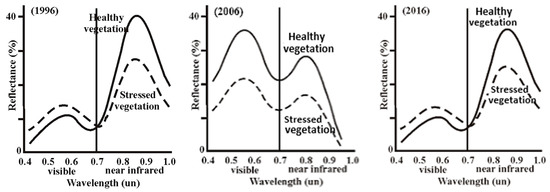
Figure 3.
Spectral reflectance of healthy and unhealthy (stressed) vegetation within the visible and infrared electromagnetic spectrums (1996–2016).
3.3. The Stimulation Analysis
Stimulation tools implemented in the IDRISI software are frequently used for prediction analysis (Eastman 2009a, b). In this study, the stimulated year (2030) was anticipated using the transition area matrix and transition probability matrix. The transition probability matrix depicts the probability that a given LAI class will transit into another LAI class. The transition area matrix depicts the total area displayed in cells or pixels (30 m × 30 m), generated by multiplying each column in the transition probability matrix with cells of the LAI in the preceding image. Table 3 is a matrix table that shows the stimulation analysis (2016–2030). Considering Table 3, we see that the rows show older LAI class categories while the column depicts newer class categories. Conditional probability maps, generated with the Markov-chain model, indicate the likelihood of a given cell (pixel) being located in a specific class in the future. Figure 4a–c show how they are used to graphically represent the transition probability matrix. The final stimulated LAI maps are depicted in Figure 5.
Table 3.
(a) Transition area matrix. (b) Cells that are expected to transition.
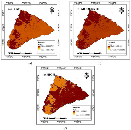
Figure 4.
(a–c) Markovian Conditional Probability maps.
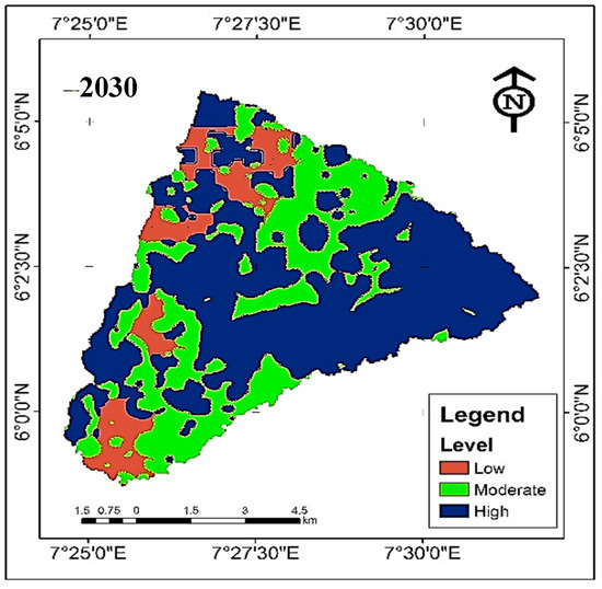
Figure 5.
Stimulated LAI maps (2030).
Table 3a displays the transition probability matrix table. The spatial–temporal analysis shows that the likelihood of LAI class 1 changing to itself is 0.2329, shifting to LAI class 2 is 0.3413, and shifting to LAI class 3 is 0.4258. The probability of LAI class 2 shifting to LAI class 1 is 0.0643, for itself it is 0.2826, and for LAI class 3 it is 0.6531. The likelihood of LAI class 3 changing to LAI class 1 is 0.0502, to class 2 is 0.2752, and to itself is 0.6746. Table 3b depicts the cells that are expected to transition to different LAI classes. Table 4 summarizes the final spatial–temporal stimulation for 2030. If we compare the analysis in Table 2 with that in Table 3, we see that in the stimulated year (2030), the health status of vegetation has rapidly declined. As vegetation becomes stressed and diminishes, it therefore implies that by 2030, more carbon will be released into the atmosphere, hence increasing climate change.
Table 4.
The spatial–temporal stimulation for 2030.
4. Conclusions
The study shows that remote sensing is an important technique for modeling and stimulating hydrocarbon micro-seepage in anomalous zones. A useful algorithm in remote sensing, known as the Leaf Area Index (LAI), has been adopted as a factor for studying the health status of vegetation. Due to the varied spatial–temporal resolutions of space satellite data, remote sensing techniques have the potential to quantify LAI fluctuations at a diverse spatial–temporal scale. The study investigates and promotes the impact of hydrocarbon micro-seepage on vegetation ecosystems in Ugwueme, Nigeria’s southern-eastern region. To achieve this aim, three cloud-free Landsat images, from Landsat TM 1996, ETM+2006, and Landsat 8 OLI 2016, were acquired from the United States Geological Survey (USGS) portal (http://earthexplorer.usgs.gov/, accessed on 4 January 2016) for the creation of low, moderate, and high LAI classification maps. The results of the study show that remote sensing technology can be effectively used to delineate areas of vegetation anomalies and alterations.
Author Contributions
Conceptualization, M.A.E. and C.O.; methodology, M.A.E.; software, M.A.E.; validation, M.A.E., C.O. and N.Y.N.; formal analysis, M.A.E. and N.Y.N.; investigation, C.O.; writing original draft preparation, M.A.E.; writing-review and editing supervision, M.A.E., C.O. and N.Y.N.; project administration, M.A.E., funding acquisition, C.O. and N.Y.N. All authors have read and agreed to the published version of the manuscript.
Funding
This research had received no external funding.
Institutional Review Board Statement
Not applicable.
Informed Consent Statement
Not applicable.
Data Availability Statement
Not applicable.
Conflicts of Interest
The authors declare no conflict of interest.
References
- Enoh, M.A.; Okeke, F.I.; Okeke, U.C. Automatic lineaments mapping and extraction in relationship to natural hydrocarbon seepage in Ugwueme, South-Eastern Nigeria. Geod. Cartogr. 2021, 47, 34–44. [Google Scholar] [CrossRef]
- Zheng, G.; Xu, W.; Etiope, G.; Ma, X.; Liang, S.; Fan, Q.; Sajjad, W.; Li, Y. Hydrocarbon seeps in petroliferous basins in China. A first inventory. J. Asian Earth Sci. 2018, 151, 269–284. [Google Scholar] [CrossRef]
- Noomen, M.F.; Van Der Werff, H.M.A.; Van Der Werff, F.D. Spectral and Spatial indicators of Botanical changes caused by long-term hydrocarbon seepage. Ecol. Inform. 2012, 8, 55–64. [Google Scholar] [CrossRef]
- Devi, A.; Boruah, S.; Gilfellon, G. Geochemical characterization of source rock from the north bank area, upper Assam basin. J. Geological. Soc. India 2017, 89, 429–434. [Google Scholar] [CrossRef]
- Bhagobaty, R.K. Hydrocarbon-utilizing bacteria of natural crude oil seepages. Digboi oil field, northern region of India. J. Sediment. Environ. 2020, 5, 177–185. [Google Scholar] [CrossRef]
- Kennicult, M. Oil and gas seeps in the Gulf of Mexico. In Habitats and Biota of the Gulf of Mexico: Before the Deepwater Horizon Oil Spill; Springer: New York, NY, USA, 2017; pp. 275–358. [Google Scholar]
- He, J.; Zhang, W.; Lu, Z. Seepage system of oil-gas and its exploration in Yinggehai basin located at NorthWest of South China Sea. J. Nat. Gas Geosci. 2017, 2, 29–41. [Google Scholar] [CrossRef]
- Garain, S.; Mitra, D.; Das, P. Mapping hydrocarbon micro-seepage prospect areas by integrated studies of aster processing, geochemistry and geophysical surveys in Assam-Arakan fold belt, NE India. Int. J. Appl. Earth Obs. 2021, 102, 102432. [Google Scholar]
- Shi, P.L.; Fu, B.H.; Ninomiya, Y.; Sun, J.; Li, Y. Multispectral remote sensing mapping for hydrocarbon seepage- induced lithologic anomalies in the Kuqa foreland basin, South Tian Shan. J. Asian Earth Sci. 2012, 46, 70–77. [Google Scholar] [CrossRef]
- Argentino, C.; Kate, A.W.; Sunil, V.; Stephane, P.; Stefan, B.; Giuliana, P. Dynamics and history of methane seepage in the SW Barents Sea: New insights from Leirdjupet fault complex. Sci. Rep. 2021, 11, 4373. [Google Scholar] [CrossRef]
- Etiope, G. Natural gas seepage. In The Earth’s Hydrocarbon Degassing; Springer: Basel, Switzerland, 2015; p. 199. [Google Scholar]
- Tangestani, M.H.; Validabadi, K. Mineralogy and geochemistry of alteration induced by hydrocarbon seepage in an evaporate formation. A case study from the Zagros Fold Belt, SW Iran. Appl. Geochem. 2014, 41, 189–195. [Google Scholar] [CrossRef]
- Giovanni, M.; Stefano, C.; Eleonora, S. Geological and Geochemical setting of natural hydrocarbon emissions in Italy. Adv. Nat. Gas Technol. 2012, 556. [Google Scholar] [CrossRef]
- Lillesand, T.M.; Kiefer, R.W. Remote Sensing and Image Interpretation, 3rd ed.; John Wiley and Sons: New York, NY, USA, 1994. [Google Scholar]
- Gitelson, A.A.; Kaufman, Y.J.; Stark, R.; Rundquist, D. Novel algorithms for remote estimation of vegetation fraction. Remote Sens. Environ. 2002, 80, 76–87. [Google Scholar] [CrossRef]
- Jin, Z.; Zhuang, Q.; Wang, J.; Archontoulis, S.; Zobel, Z.; Kotamarthi, V. The combined and separet impacts of climate extremes on the current and future US rainfed maize and soya-bean production under elevated CO2. Glob. Chang. Biol. 2017, 23, 2687–2704. [Google Scholar] [CrossRef]
- Enoh, M.A.; Okeke, U.C.; Barinua, N.Y. Modelling and delineation of hydrocarbon micro-seepage prone zone on soil and sediment in Ugwueme, South-Eastern Nigeria with Soil Adjustment Vegetation Index (SAVI). Int. J. Plant Soil Sci. 2020, 32, 13–33. [Google Scholar] [CrossRef]
- Wang, Z.; Qi, Z.; Xue, L.; Bukovsky, M.; Helmers, M.J. Modeling the impacts of climate change on nitrogen losses and crop yield in a subsurface drained field. Clim. Chang. 2015, 129, 323–335. [Google Scholar] [CrossRef]
- Aly, A.A.; Al-Qmran, A.M.; Sallam, A.S.; Al-Wabel, M.I.; Al-Shayann, M.S. Vegetation cover change detection and assessment in arid environment using multi-temporal remote sensing images and ecosystem management approach. Solid Earth 2016, 7, 713–715. [Google Scholar] [CrossRef]
- Fogwe, Z.N.; Tume, S.J.; Fouda, M. Eucalyptus Tree Colonization of the Bafut-Ngemba Forest Reserve, North West Region, Cameroon. Environ. Ecosyst. Sci. 2019, 3, 12–16. [Google Scholar] [CrossRef]
- Huete, A.R. A soil-adjusted vegetation index (SAVI). Remote Sens. Environ. 1988, 25, 295–309. [Google Scholar] [CrossRef]
- Breda, N.J. Ground-based measurements of leaf area index: A review of methods, instruments and current controversies. J. Expermintal Bot. 2003, 54, 2403–2417. [Google Scholar] [CrossRef]
- Jonckheere, I.; Fleck, S.; Nackaerts, K.; Muy, B.; Coppin, P.; Weiss, M.; Baret, F. Review of methods for in situ leaf area index determination: Part I. Theories, sensors and hemispherical photography. Agric. For. Meteorol. 2004, 121, 19–35. [Google Scholar] [CrossRef]
- Weiss, M.; Baret, F.; Smit, G.; Jonckeere, I.; Coppin, P. Review of methods for in situ leaf area index (LAI) determination: Part II. Estimation of LAI, errors and sampling. Agric. For. Meteorol. 2004, 121, 37–53. [Google Scholar] [CrossRef]
- Chen, J.M. Remote sensing of leaf area index of vegetation covers. In Remote Sensing of Natural Resources; CRC Press: Boca Raton, FL, USA, 2013; pp. 375–398. [Google Scholar]
- Parsa, V.A.; Yavari, A.; Nejadi, A. Spatio-temporal analysis of land use and land cover pattern changes in Arasbaran Biospshere Reserve, Iran. Model. Earth Syst. Environ. 2016, 2, 178. [Google Scholar]
- Teferi, E.; Bewket, W.; Uhlenbrook, S.; Wenninger, J. Understanding recent land use and land cover dynamics in the source region of the Upper Blue Nile, Ethopia. Spatially explicit statistical modelling of systematic transitions. Agric. Ecosyst. Environ. 2013, 165, 98–117. [Google Scholar] [CrossRef]
- Thomas, H.; Laurence, H.M. Modelling and projecting land-use and land-cover changes with a cellular automation in considering landscape trajectories: An improvement for simulation of plausible future states; EARsel. EARSeL eProceedings 2006, 5, 63–76. [Google Scholar]
- Guan, D.; Gao, W.; Watari, K.; Fukahori, H. Land use change of Kitakyushu based on landscape ecology and Markov model. J. Geogr. Sci. 2008, 18, 455–468. [Google Scholar] [CrossRef]
- Ma, C.; Zhang, G.Y.; Zhang, X.C.; Zhao, Y.J.; Li, H.Y. Application of Markov model in wetland change dynamics in Tianjin Coastal Area, China. Procedia Environ. Sci. 2012, 13, 252–262. [Google Scholar] [CrossRef]
- Subedi, P.; Subedi, K.; Thapa, B. Application of a hybrid cellular automation Markov (CA-Markov) model in land-use change prediction. A case study of saddle creek drainage Basin, Florida. Appl. Ecol. Environ. Sci. 2014, 1, 126–132. [Google Scholar]
- Singh, S.K.; Mustak, S.; Srivastava, P.K.; Szabo, S.; Islam, T. Predicting spatial and decadal LULC changes through Cellular Automata Markov Chain Models using earth observation datasets and geoinformation. Environ. Process. 2015, 2, 61–78. [Google Scholar] [CrossRef]
- Guan, D.; Li, H.; Inohae, T.; Su, W.; Nagaie, T.; Hokao, K. Modelling urban land use change by integration of cellular automation and Markov model. Ecol. Model. 2011, 222, 3761–3772. [Google Scholar] [CrossRef]
- He, D.; Zhou, J.; Gao, W.; Guo, H.; Yu, S.; Liu, Y. An integrated CA-Markov model for dynamic simulation of land use change in Lake Diachi watershed. Bejing Daxue Xuebao (Ziran Kexue Ban)/Acta Sci. Nat. Univ. Pekin. 2014, 50, 1095-05. [Google Scholar]
- Liping, C.; Yujun, S.; Saeed, S. Monitoring and predicting land use and land cover changes using remote sensing and GIS techniques. A case study of a hilly area, Jiangle, china. PLoS ONE 2018, 13, e0200493. [Google Scholar] [CrossRef] [PubMed]
- Yang, X.; Zheng, X.C.; Chen, R. A land-use change model. Integrating landscape pattern indexes and Markov-CA. Ecol. Model. 2014, 283, 1–7. [Google Scholar] [CrossRef]
- Memarian, H.; Balasundran, S.K.; Talib, J.B.; Sung, C.T.; Sood, A.M.; Abbaspour, K. Validation of CA-markov for simulation of land use and land cover change in the Langat basin, Malaysia. J. Geographic. Inf. Syst. 2012, 4, 542–554. [Google Scholar] [CrossRef]
- Hyandye, C.; Martz, L.W. A Markovian and Cellular Automata Land-Use Change Predictive Model of the Usangu catchment. Int. J. Remote Sens. 2017, 38, 64–81. [Google Scholar] [CrossRef]
- Blackburn, G.A. Hyper-spectral remote sensing of plant pigments. J. Exp. Bot. 2007, 58, 855–867. [Google Scholar] [CrossRef] [PubMed]


Disclaimer/Publisher’s Note: The statements, opinions and data contained in all publications are solely those of the individual author(s) and contributor(s) and not of MDPI and/or the editor(s). MDPI and/or the editor(s) disclaim responsibility for any injury to people or property resulting from any ideas, methods, instructions or products referred to in the content. |
© 2022 by the authors. Licensee MDPI, Basel, Switzerland. This article is an open access article distributed under the terms and conditions of the Creative Commons Attribution (CC BY) license (https://creativecommons.org/licenses/by/4.0/).