1. Introduction
Geometry is widely used in aviation, from designing airfoils to implementing procedures. For its part, statistics plays a key role for traffic forecasting and predictive maintenance. Yet, contrary to geometry, statistical analyses of aircraft trajectories have been under-exploited in the Airspace Traffic Management (ATM) literature. One possible reason is the irrelevance of usual statistical frameworks to model a trajectory. Indeed, techniques from multivariate statistics suffer from the very high correlation in time that exists between two consecutive points of a trajectory. More worryingly, when observation times are more numerous than the number of trajectories, the so-called curse of dimensionality occurs. Nor is the usual time-series approach ideal, as trajectories can be seen as multidimensional time series with both irregular sampling and different durations.
The current institutional context evolves towards a greater availability of trajectory data. On the one hand, Eurocontrol has given access to a R&D data archive containing more than 17 million flights as of April 2022. On the other hand, the non-profit OpenSky Network has grown to 5000 registered receivers all around the world, providing a large historical database of ADS-B data that is accessible to researchers [
1].
Interestingly, past OpenSky Network symposia have demonstrated how statistics could provide some solutions to complex problems such as trajectory generation [
2] or pattern identification [
3], encouraging the development of new statistical methods to model trajectories.
An adapted statistical framework to study trajectories is the one of Functional Data Analysis (FDA), popularized by [
4,
5]. Early promotion of FDA to study aircraft trajectories was made by [
6]; it has been successfully used for Functional Principal Component Analysis (FPCA) by [
7] and applied to the detection of atypical energy behaviors by [
8].
Recently, FDA has progressively made the most of differential geometry to study any kind of trajectory. As an example, Ref. [
9] analyzed bird and hurricane trajectories on Riemannian manifolds. Incorporating geometry in statistics is particularly relevant for at least two reasons. First, parametric curves are naturally good descriptors of motion. This makes geometry a perfect framework to describe a dynamic system evolving over time. Second, geometry allows the careful study of the shape of a trajectory under arbitrary temporal evolution, taking into account translation, scale and rotational effects.
This work introduces a number a geometrical methods to quantify how the shape of a given trajectory changes from the R&D archive version to the ADS-B one. In addition to providing a proper shape-based distance between the two versions, we compute the optimal deformation required to go from the R&D archive version to the ADS-B one. In other words, a geodesic path allows to visualize all the bending and stretching transformations that are necessary to go from one version to the other.
Far from being purely theoretical, the presented geometric framework has many operational applications. In this work, the geodesic distance enables both the visualization and quantification of where and how much the flown trajectory has diverted from the flight plan. The geodesic distance is also used to solve a clustering problem based on shape.
This paper first introduces the geometric framework of shape analysis, departing from the early work of Kendall and coauthors to more recent methods. Second, the geodesic distance is defined. Third, a sample of flights is used to illustrate how the R&D archive version of a trajectory (Eurocontrol) changes from its ADS-B version (OpenSky Network).
2. What Is the Shape of a Trajectory?
Whichever the data provider (Eurocontrol or OpenSky Network), a raw trajectory
associated to a flight index
i is a set of
pairs:
where
is the number of observation times associated with flight index
i,
is a three-dimensional vector (longitude, latitude and altitude), and
is a timestamp. In what follows, the components of
are, respectively, denoted
,
,
. We need to determine how to define the shape of such an object and what we mean by shape in the first place.
One of the earliest works in statistical analysis and modeling of shapes of objects came from Kendall and colleagues [
10,
11]. Their adopted definition of a shape is still commonly used in geometry and statistics. As defined by [
12], a shape is all the geometrical information that remains when location, scale and rotational effects are removed from an object. Two objects have the same shape if they can be translated, rescaled and rotated to each other so that they match exactly.
Whatever the nature of objects under study (images, sounds, curves, or surfaces), shape was originally described by locating a finite number of points on each object. These so-called landmarks are points of correspondence and can be assigned by an expert (scientific landmark) or suggested by a property of the object, such as a point of high curvature (mathematical landmark). The positions of these landmarks are points in . It is often assumed that the number of landmarks k is greater than or equal to the dimension n. The configuration is the set of landmarks on a particular object. The configuration matrix X is the matrix of the Cartesian coordinates of k landmarks in n dimensions. The configuration space is the space of all landmark coordinates, usually the space of real matrices with possibly some special cases removed, such as coincident points. This space is denoted . Within the same shape class, many configurations are possible. Indeed, two objects have the same shape if their configurations are equivalent. These variations are formulated as actions of certain groups. In shape analysis, usual variations are all actions of Lie groups—that is to say, mathematical objects that are both a group and a differential manifold. Lie groups of interest are the translation group , the scaling group and the rotation group . The three variations are combined together considering a product group denoted , where ⋊ is the semi-direct product.
The action of on is , where is a column vector of length k containing all ones so that is a matrix with identical columns given by v. More specifically, landmark space analysis relies on the study of spaces of equivalence classes, which are called quotient spaces in differential geometry. The quotient space of interest is and is termed the landmark shape space. In quotient space live orbits. In differential geometry, for any element p of a manifold M, the orbit of p under the action of group G is defined as the set and is written . The orbit of a point in a manifold refers to all possible points one can reach in the manifold using the action of the group on that point.
Landmark shape analysis has led to many practical applications. In biology, it has been used to quantify the effects of selection for body weight on the shape of mouse vertebrae [
13] and to highlight sexual dimorphism in hominoids using craniofacial shape differences [
14]. In chemistry, Refs. [
15,
16] analyzed a dataset of steroids to evidence how the shape (“steric”) properties of the molecules are related to an activity class.
Despite these successful applications, the use of landmarks is not straightforward for the study of aircraft trajectories for at least three reasons:
The choice of landmark is very subjective. How many landmarks are relevant to summarize the shape of an aircraft trajectory? Should this number depend on the origin–destination we consider? Would landmarks based on flight phases be enough to capture the shape of a trajectory?
Scientific landmarks are not available in raw data. Both Eurocontrol and OpenSky Network data sources do not include expert knowledge.
Mathematical landmarks are likely to be imprecise for Eurocontrol data. Indeed, recovering flight phases thanks to existing algorithms ([
17] or [
18]) will perform differently depending on the number of observation points.
These limits are not new. They were exemplified in medical imaging problems for which landmarks are not obvious to find (think of soft tissues where boundaries have no sharp edges). These problems were taken into account by [
19] in the same spirit as Kendall’s formulation, one of the first attempts to propose a convenient shape representation of curves in
. This is the framework we consider in the sequel.
3. Trajectories as Parameterized Curves in
As said, raw data are stored in a usual matrix format. A few preliminary remarks should be made. First, the duration changes from one flight to another. As a consequence, the number of observation points in not the same from one trajectory to another. Second, for a given trajectory, observation times are not equally spaced. Third, between two trajectories, the spacing is irregular but is never the same. For a given trajectory, observation points are the same for all components of .
Given that most methods in time-series and multivariate statistics are inappropriate in this context, a relevant statistical framework is to study trajectories from a Functional Data Analysis (FDA) perspective. The main assumption in FDA is the existence of an underlying function that has given birth to a set of values the statistician observes on the aforementioned irregular grid. When the number of observations is high enough, each underlying function is retrieved thanks to interpolation or smoothing. It is then effortless to resample trajectories on a regular grid.
In FDA, a trajectory is viewed as the realization of a functional random vector. A functional random vector of dimension p is denoted . Note that . More precisely, each component is a functional random variable taking its values in an infinite dimensional vector space, often chosen to be associated with the scalar product for .
As the three dimensions of a trajectory (longitude, latitude and altitude) are based on an underlying coordinate system, once reconstructed, a trajectory can be viewed as an open parameterized curve of .
As each trajectory has a different duration, scaling is made so that each curve goes from to .
3.1. Interpolation: From Raw Data to Curves
Going from raw data to smooth curves calls for a smoothing or interpolation step. Smoothing refers to the case in which observations are assumed to be noisy, whereas interpolation hypothesizes that observations are recorded with negligible errors. Many smoothing and interpolation methods are available to reconstruct individual trajectories. A review of four popular non-parametric techniques is given in [
20]. Whatever the method, the construction of functional observations using the discrete data takes place separately for each dimension of a flight: the longitude, the latitude and the altitude.
Linear interpolation is chosen in this work because Eurocontrol R&D data are based on updated filled flight plans, in other words, a series of straight lines.
3.2. The Square-Root Velocity Function (SRVF) Captures Shape
Once trajectories are interpolated, their shape can be studied. To this end, the Square-Root Velocity framework has been developed in [
19]. The main assumption is that curves are differentiable with a first derivative in
. In this framework, the shape of a curve is no more captured by landmarks but by the Square-Root Velocity Function (SRVF). Let
be a mapping given by:
where
denotes the usual Euclidean norm of
. The SRVF of
is defined to be
, where
is the time gradient of
. The curve
can be reconstructed from
q up to a translation. Luckily, the SRVF naturally removes translation effects as it is based on the curve derivative.
Scale effects are easy to remove, as all curves can be rescaled to be of unit length in a preprocessing step.
The space of interest is then
It is the set of all Square-Root Velocity Functions with unit
-norm. As recalled in [
21], this corresponds to a sphere in
. A lot is known about the geometry of such a sphere, including geodesics. Shape analysis of curves under this representation (without additional constraints) is relatively simple. Yet we still need to take care of different re-parameterizations of curves as well as the effect of rotations.
3.3. How to Deal with Rotation and Re-Parameterization
The action of the rotation group is usual and similar in landmark-based shape analysis: , .
Yet parameterization effects are specific to the Square-Root Velocity (SRV) framework because there is no parameterization in the landmark-based approach. Note that it is natural that shape should be invariant by re-parameterization: two curves may have the same shape but be traveled along at a different pace.
In the SRV framework, a re-parameterization is an element of , the set of all orientation-preserving diffeomorphisms of . Orientation-preserving means that the transformed passage of time is still coherent (time is not moving back: 0 maps to 0 and 1 maps to 1). Working with diffeomorphisms allows us to actually re-parameterize curves. For a , the composition denotes its re-parameterization. It can be shown that the associated group action is , .
The quotient space of interest is
. Crucially, Ref. [
19] have shown that if the Riemannian metric is well-chosen to be an elastic Riemannian metric, the rotation group
and the re-parameterization group
both act by isometries. This property is key to define distances between orbits, that is to say, distances between elements of the quotient space.
is called the shape space and is a metric space with the distance inherited from
. It is a collection of orbits (individual shapes):
.
3.4. Distance between Two Shapes, Geodesic Path
The distance between two orbits
and
is given by:
with
, where
is the usual inner product between vectors in
.
The actual geodesic between
and
in
is given by
, where
is the geodesic in
between
and
. Computing
is very easy because
is a sphere.
and
minimize the right side of the above distance. This is a joint optimization problem with a well-known solution, as pinpointed in [
21].
4. Application
4.1. Data
4.1.1. R&D Eurocontrol
Eurocontrol is an international organization working to achieve safe and seamless air traffic management across Europe. Since 2020, Eurocontrol has given access to a R&D data 192 archive containing more than 17 million flights as of April 2022. The data are collected from all commercial flights operating in and over Europe. To be more specific, Eurocontrol receives flight plans for all Instrument Flight Rules (IFR) flights. These flight plans are activated and updated based on live data from air navigation service providers. Data are available for 4 months each year: March, June, September and December. Only two data subsets are used in this work: flight metadata and actual flight points. We are interested in studying the 15,628 flights that departed from Toulouse–Blagnac (LFBO) and landed at Paris–Orly (LFPO) from March 2015 to March 2020.
In the R&D data archive, all flights are identified by a unique code coming from the PRISME Data Warehouse (DWH). The registration number is also available. There are 386 unique registration numbers for the 15,628 flights.
The actual off-block time as well as the actual arrival time, respectively, correspond to the first and last points of a trajectory.
4.1.2. Retrieving ADS-B Flights Thanks to OpenSky Network
To query a flight in the OpenSky Network database (Impala Shell), one should use an ICAO24 identifier and a date. The ICAO24 code is a unique 24-bit number that is assigned to each vehicle or object that can transmit ADS-B messages. The correspondence between the registration number and the ICAO24 code is made thanks to the aircraft database of the OpenSky Network. Among the 15,628 flights, only 999 cannot be matched.
To find a flight in the OpenSky Network flight table, the query is made using the actual off-block time and the actual arrival time with an additional time buffer. A query outputs several candidate flights.
The proportion of flights for which there is at least one candidate goes from 0% in 2015 (this was expected, as ADS-B data were not collected by OpenSky Network in 2015) to 85% in 2018. For each Eurocontrol flight, the ADS-B flight that is most likely (same ICAO code and closest off-block time) is kept. At this step, 6053 flights remain. State vectors are then queried with a time buffer. Thus, 6031 flights remain.
A great challenge when matching ADS-B data and Eurocontrol data is the problem of the beginning/end of a flight. The two first points of any flight in the R&D archive are located at the same geographical coordinates (the ones of the departure airport) with zero altitude. The time between the first two points is most likely the actual taxi-out time, that is to say, the period between the actual off-block time and the actual take off time. As the taxi-out time is not visible with ADS-B data, the first point of any flight from the R&D archive is removed. Duration is computed as being the time difference between the first point and the last point of the flight.
ADS-B data can be very noisy. Some basic filters are used to withdraw outliers. For instance, ADS-B flights with fewer than 20 points are withdrawn. ADS-B flights for which there is at least one time gap between two points that exceeds 20 min are withdrawn. A total of 5226 flights remain after the cleaning step.
In the spirit of the ADS-B cleaning step, Eurocontrol flights with fewer than 10 points are removed from the analysis, as well as flights having a time gap between two consecutive points that is at least 20 min. A total of 5180 trajectories remain after this step.
4.2. Interpolation
In total, there are 5180 flights for which we have both a clean ADS-B version and a clean corresponding Eurocontrol version. For example, in 2019, there are 1746 valid trajectories.
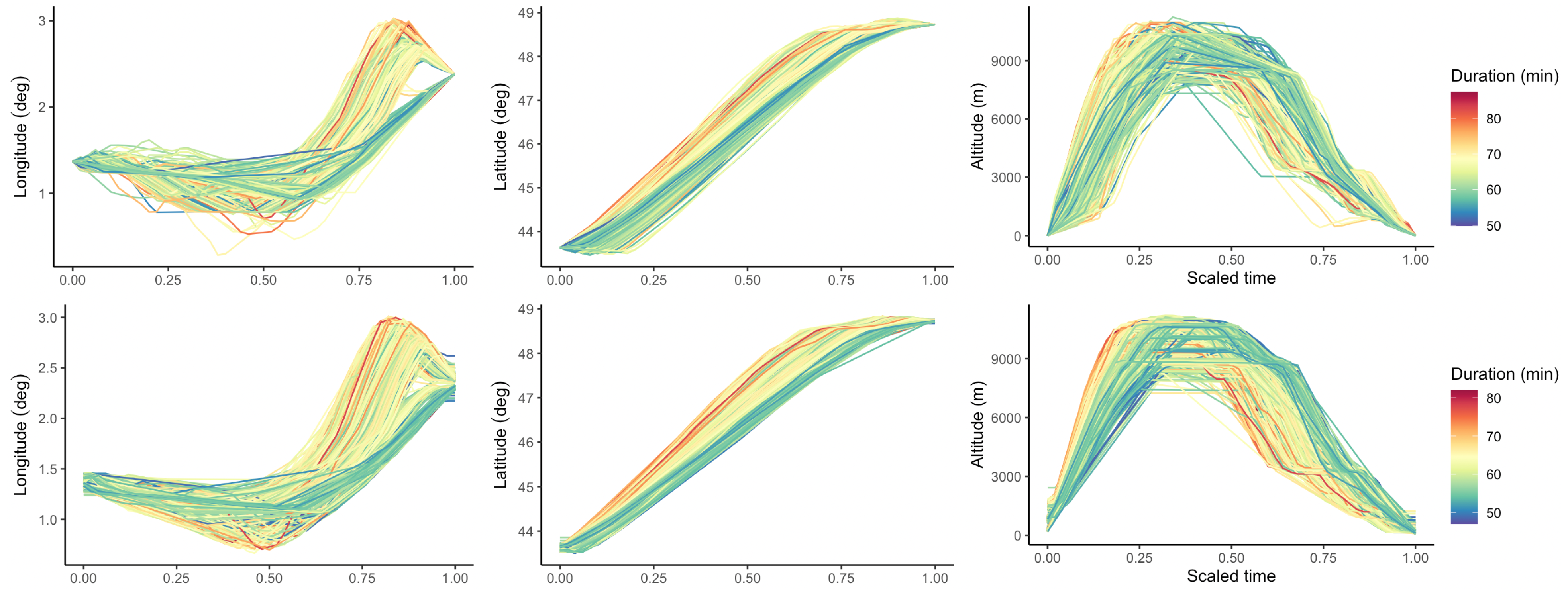
Interpolation is done year-by-year and an example for the year 2019 is given in
Figure 1. For both Eurocontrol and ADS-B data, the linear interpolation resamples all trajectories on a regular grid ranging from 0 to 1 with an incrementation of 0.02.
Contrary to the altitude profiles of Eurocontrol trajectories, the take-offs and landings of ADS-B trajectories are not always associated with a null altitude. This phenomenon and the small difference between the two color scales come from the aforementioned problem of finding the true beginning/end of an ADS-B flight.
As expected,
Figure 2 shows a striking difference between the shape of trajectories from their ADS-B version to their Eurocontrol one.
4.3. How to Compute the Geodesic Path in Practice
Most geometric concepts developed by [
19,
22] have been implemented in R in the
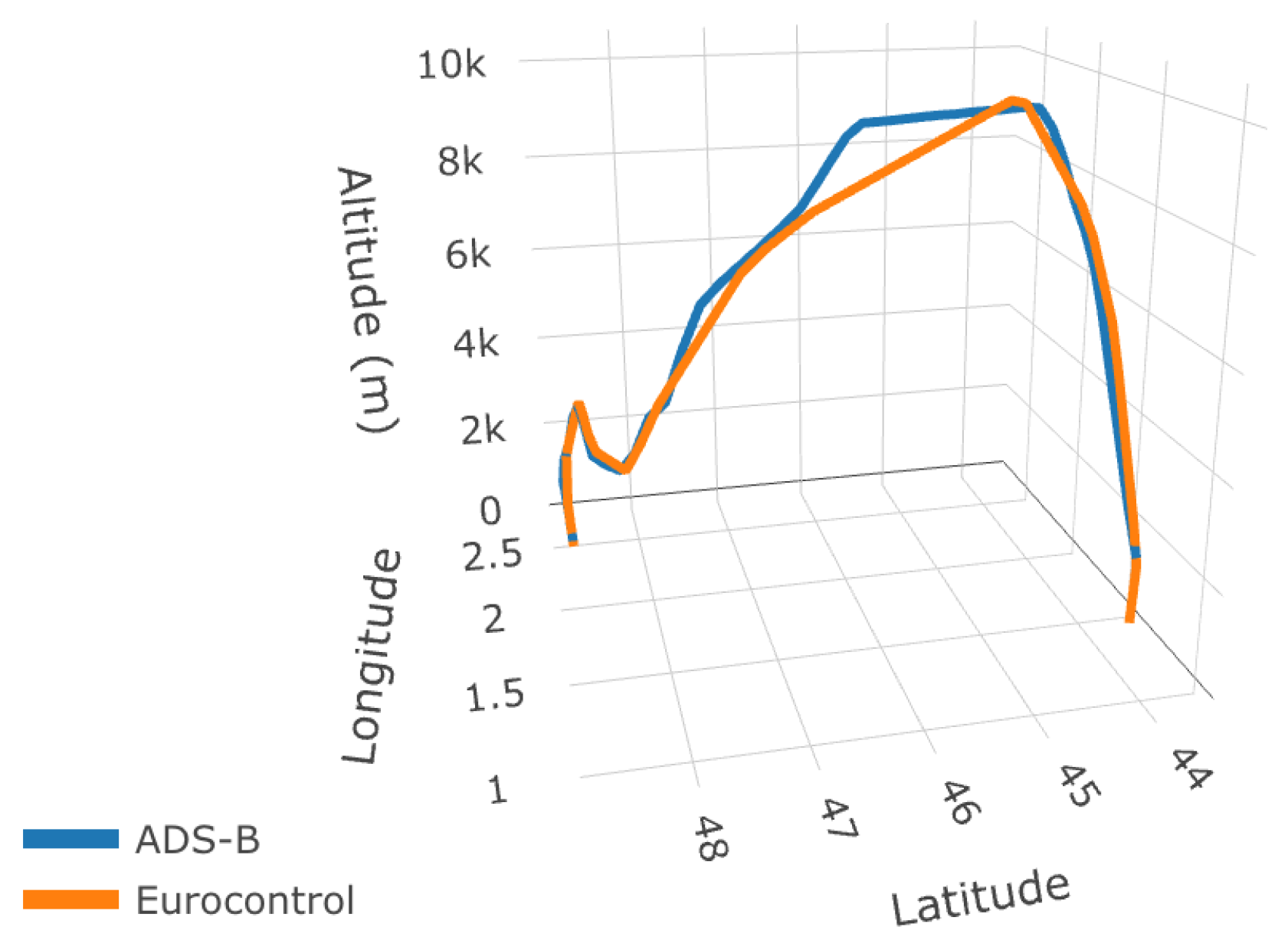
fdasrvf package maintained by J. Derek Tucker. Computation of the geodesic path for a given flight is illustrated in
Figure 3.
Once re-parameterization, location, scale and rotational effects have been taken into account, bending and stretching transformations are necessary to match the two versions. One possible representation of the shortest (in the quotient space) is shown in
Figure 4.
4.4. Geodesic Distance
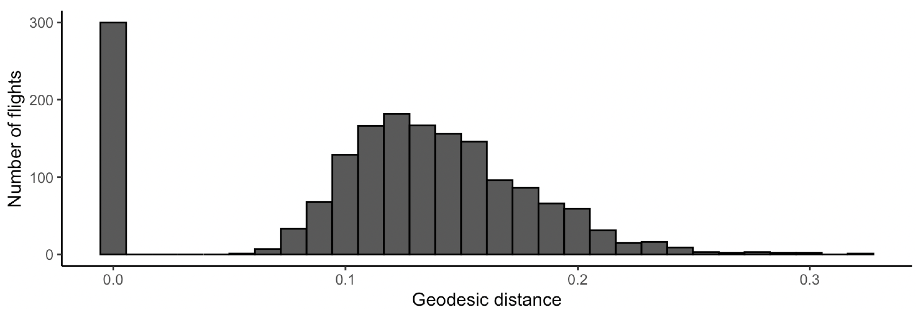
The histogram in
Figure 5 clearly shows two groups of flights. When the geodesic distance is null, no bending/stretching is needed to match trajectories once location, scale, rotational and re-parameterization effects are taken into account. In this case, Eurocontrol and OpenSky versions are carrying the same shape information. Yet this is not the case when the geodesic distance is not null. In most cases, one should benefit from OpenSky Network ADS-B data, as these are more detailed.
4.5. Hierarchical Clustering
The geodesic distance may be used for the clustering and classification of trajectory shapes. As an example, Refs. [
19,
21] have successfully clustered shapes of helices in
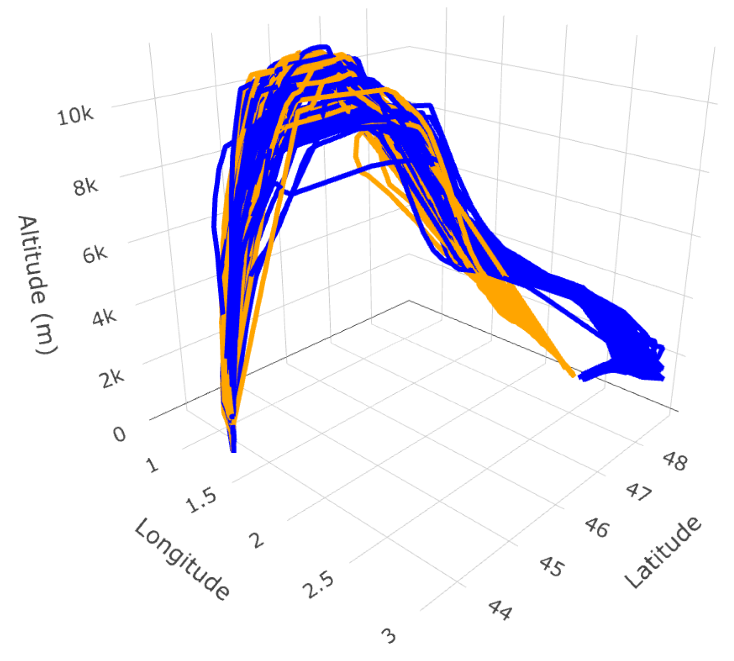
by matching and deforming one into another, the underlying motivation being the analysis of protein structures. In a similar spirit, clustering of ADS-B trajectories based on their shapes can be performed. In this section, a random sample of 100 trajectories departing from Toulouse–Blagnac (LFBO) and landing at Paris–Orly (LFPO) in 2019 is drawn. Hierarchical clustering is implemented. The geodesic distance matrix is computed, and Ward’s method is chosen to perform the clustering. When the quotient space we consider is taken to be
(translation, scale, rotational and re-parameterization effects are removed), shape clusters are mostly based on the arrival direction at Paris–Orly airport (LFPO), as one may note from
Figure 6.
5. Discussion
The growing availability of ADS-B data is likely to have a huge impact on statistical studies. As compared to the Eurocontrol R&D data archive that is based on updated filled flight plans, ADS-B data allow for reliable studies of shapes. Tools from differential geometry, namely the geodesic distance, help to quantify and clarify empirical assessments of how far flown trajectories are from the flight plan. This distance can be used in clustering problems.
This paper focused on a sample of flights that is not representative of all flights in Europe. Future work may quantify the benefits of ADS-B data for each flight phase and for a larger scope. The parsimonious sampling of Eurocontrol R&D data is likely to be satisfactory for shape analysis focusing on the en-route phase.
In this work, the ADS-B cleaning process is basic and should be refined in future work. Matching Eurocontrol flights with their ADS-B versions is far from trivial and requires in-depth study.
Depending on operational needs, the quotient space defining what is meant by shape should be modified. An interesting extension could be to investigate the relevant geometrical framework needed to model go-around patterns.


