On the Prospective Use of Deep Learning Systems for Earthquake Forecasting over Schumann Resonances Signals ^†

Abstract

The relationship between Schumann resonances and earthquakes was proposed more than 50 years ago; however, the experimental support has not been fully established. A considerable amount of recent studies have focused on the relationship between a single earthquake and the Schumann resonance signal variation around this earthquake, obtaining preliminary support for the existence of the link. Nonetheless, they all lack a systematic and general approach. In this research, we propose a novel methodology to detect the presence of relevant earthquakes based on the Schumann resonance. The methodology is based on a deep learning framework composed of a pretrained variational auto-encoder followed by an LSTM network and a fully connected layer with a sigmoid output. The results reveal the uncovered relationship between earthquake activity and Schumann resonance signal using the novel methodology, being the first automatic earthquake detector based on Schumann resonance signal.

1. Introduction

Schumann resonance (SR) are extremely low frequency (ELF) electromagnetic signals generated mainly through the lightning iteration, which propagates along the Earth–ionosphere Electromagnetic Cavity [1]. The electromagnetic cavity is formed by two electromagnetic media with a high level of conductivity (the Earth and the ionosphere) and an insulator (the atmosphere). The electromagnetic resonance produced has multiple modes in which the intensity of higher modes are considerably lower than the first modes [2]. Experimentally, the average central frequency for the first six modes is agreed to be around 7.8 Hz, 14 Hz, 20 Hz, 26 Hz, 33 Hz, and 39 Hz. Despite that, no theoretical characterization of the frequency of the SRs modes manages to accurately fit the experimental results. For example, in [3], the authors detailed a novel method for estimating the central values; however, the results do not agree accurately with the experimental worldwide data. Other studies have approached the central frequency estimation using a 3D electromagnetic simulator with very promising results [4,5]. Although the results are consistent with the experimental data, they are not completely equal to them. It is important to remark that all these approaches are centered on the central frequency estimation in a steady condition, the analytical or simulated behavior of the SR frequency variation remains undiscovered.

In light of the above, it is clear that there is difficulty involved in the estimation of the SR signal parameters, even for one of the simplest parameters, e.g., the central frequency for the first mode in the steady condition. This fact has led this team to introduce deep learning (DL) techniques in order to analyze it.

Over the last five years, one of the most studied parts of SR has been the diurnal and seasonal patterns of SR and their evolution over the time. The importance of this pattern is mainly driven by the fact that many observatories have been set up during these years. The diurnal and seasonal patterns of a UK observatory is fully explained in [6]. They explain the specific frequency registered by their observatory based on the proximity to the African thunderstorm. In [7], the researchers detailed this regular pattern and its relation with the most important lightning hot spots during specific hours of the day. Slight differences are also expected between observatories. Some aspects of the electromagnetic composition of the Earth–ionosphere cavity can be explained based on the little differences between observatories. For example, in [1], the authors use two distant stations and focus on the comparison between their spectrum and the differences between the central frequency of the first mode. In recent years, a growing interest in their relationship with other natural phenomena has received more attention; for example, the connection with the lightning activity [8,9], the relation with geomagnetic storms in [10], or with a solar proton event in [11]. Due to the complexity of the SR signals, the characteristics of the previously mentioned relationship have not been dealt with in depth, although the auspicious results point out a highly possible connection.

In relation with the presented research, earthquake (EQ) detection using SR signals has become a central issue in the last five years in the SR research. Experiments on detecting individual EQ were performed in the last two years with encouraging results. Some papers have centered their investigation on the relationship between individual events and their impact on the SR signal.

The study of the relation with two huge EQs in Japan is presented in [12]. The results discussed the effect of EQs both in the transient domain and in the frequency domain, along with a compelling theoretical explanation. In [13], the researchers point out the statistical link between frequency and intensity values of the first SR mode around individual seismic events. The work was centered on the study of the SR signal variations around important EQs, fifteen days before and five days after each EQ event. The study of the relation between two important EQ and their affectation in the SR signal in Greece can be found in [14]. They exposed the statistical interconnection between these two EQ events and the variation of the ELF background signal. Although this approach is interesting, it does not allow for establishing a systematical methodology that can detect EQ events using the continuous SR signal.

Other authors have focused on describing the prerequisites and modeling the electro-magnetic (EM) iteration between SR signal and EQ. A model treatment to estimate the EQ magnitude based on the variation of the SR spectrum is fully explained in [15]. The results show substantial evidence of the usage of SR signal variation for detecting EQ above 7 and at a distance up to 3 Mn. A model of the electromagnetic manifestation in the SR band by close EQ events is described in [16]. The most promising result that emerges from their research is that nearby EQs provoke noticeable modification of the SR signal. In [17], the authors studied the prerequisites to record seismic activity in the SR band in the time domain. The results using two distant stations are promising; however, the system does not fulfill the needed accuracy for the EQ prediction. The study of the possibility of forecasting EQ using a narrow transient window is explored in [18], with a machine learning (ML) approach.

To the best of our knowledge, the evidence proposed by these studies are not conclusive. The detection of EQ events is mainly performed by the analysis of individual EQ; however, a more generalized framework would be needed to established an experimental link between SR and EQ.

It is also important to mention the lack of previous studies exploring the usage of the latest advances in computational intelligence applied to SR signals, which is more than important due to the vast amount of data and the difficulty involved in detecting variation in the regular patterns, as was mentioned before.

This research presents a new approach to exploring the possibility of using the time evolution of the SR signal to detect the occurrence of high-intensity nearby EQs. The methodology is constituted of three parts: A pretrained variation auto-encoder (VAE) focuses on reducing the data dimension, followed by a long short-term memory (LSTM) network, with the aim of taking into account the temporal trend of the SR codified data and a fully connected layer to classify the interaction based on the LSTM neuron states. The aim of this paper is to use the DL advances to design a method for establishing a correlation between SR signal and EQ.

2. Materials and Methods

The methodology used in this research is composed by a deep encoder followed by an LSTM for studying the correlation between the EQ and the SR signal. A complete description of the methodology can be seen in Figure 1.

The SR signal is obtained by the ELF Sierra de Los Filabres observatory. The observatory has been recording SR signals continuously from 2016, although, due to maintenance problems, some registers were not captured. This observatory contains two sensors, one for the ${\mathcal{H}}_{NS}$ and the other for the ${\mathcal{H}}_{EW}$. The digital part is composed of an ADC with 24 bits of resolution and 187 samples per second. A detailed description of the observatory can be found in [19]. The data are recorded in 30-min segments. Each segment is processed and the Welch algorithm fetches the spectral information of each segment. Finally, each segment is reduced to a 256 length vector, which contains the frequency information from 0 $\mathrm{Hz}$ to 42 $\mathrm{Hz}$. For the sake of concreteness, we have selected only the ${\mathcal{H}}_{NS}$ sensor. Considering the data from January 2016 to December 2020, the total number of 30-min intervals is 87,697; however, due to the maintenance problem, the real number of 30 min intervals is 79,281.

The EQ data have been obtained through a public EQ Repository [20]. The total number of EQ with a Richter magnitude greater than 4.5 during the five year period is 35,023; however, not all EQs have been considered for this research, as the system will be focused on detecting the EQ, which can have more impact on the SR of our observatory. The EQ events have been filtered by an ad hoc criterium based on the expert knowledge of this group and the previous literature:

• Richter magnitude greater than 5.0.
• Distance between the EQ and the observatory less than 30 $\mathrm{k}$$\mathrm{m}$.
• Depth less than 40 $\mathrm{k}$$\mathrm{m}$.

By selecting only the EQ that fulfills these criteria, the number of EQ is reduced to 161.

The time step used in this paper is 30 min due to the resolution of the SR signal. Consequently, the EQ event has been adjusted to its corresponding 30 min time step. The duration of the EQ has been widened to 24 h, which means 48 registers around the actual event. This widened process is performed to allow the DL model to learn about the influence of the EQ on the SR signal; therefore, the widened register can no longer be considered the EQ event, but we consider the positive values as a representation of the EQ affection in the SR register.

To sum up, the ground truth comprises 87,697 registers, in which, 5459 are labeled as 1 (meaning that an EQ affected the SR register) and 82,238 are labeled as 0 (no affection).

The data set has been split into two parts:

• Training data set: from January 2016 to June 2019—60,129 samples.
• Test data set: from July 2019 to December 2020—27,568 samples.

The first step in our methodology is the usage of a pretrained DL encoder, framed in a VAE methodology. A schematic representation can be seen in Figure 2. The deep encoder is composed of three convolutional layers and two fully connected layers. The first convolutional layer takes a 1D vector of 256 positions and outputs 32 vectors of length 128. The second convolutional layer outputs 64 vectors of length 64. The last convolutional layer converts the input to 64 vectors of length 32. The last part of the encoder is composed of two fully connected layers that take the output of the last convolutional and output a code vector of 10 components. The code data set is composed of 87,692 codes of 10 values, out of which 79,281 are the output of the deep encoder plus 8000 zeros codes, which correspond with the SR lost segments due to maintenance problems. The main purpose of using the encoder is to focus on the variability of the signal, but not to take into account the common structure of the SR signal. The method selected for this purpose is a VAE, which tries to reconstruct the original signal but reduces the dimension of the input from 256 to 10; however, retaining the most critical information, while removing the record’s common part. The variational term refers to the randomization of the learned space [21]. The VAE is also reinforced by the Lorentzian fit algorithm in the cost function.

The next step is composed of an LSTM network, which sequentially takes the inputs composed by the five-year outputs of the DL encoder. The LSTM architecture is composed of an LSTM layer with 32 features in the hidden state. The LSTM network is fed with 1440 values, which correspond to 30 days of 30-min segments. After the 1440 sequence registers have been introduced into the LSTM network, the hidden state of the network is processed by a fully connected layer made of two layers. The first layer takes 32 values as the input and produces a vector of 128 values as output. The last layer processes the 128 values and outputs a code of only 1 value. In order to calculate a binary output, the last layer is followed by a sigmoid function.

The binary output of the LSTM layer is compared to the SR affectation of this register. The DL LSTM system is trained to predict the affectation of the EQ in the first 25% of the 1440 sequences. In Figure 3, a description of our LSTM methodology is outlined. The sequence is compared after 1440 values have been fed to the network (30 days). The result is compared against the EQ affectation of the 360 registers (7.5 days). In order to add more generalization to the model, an L1 regularization and a dropout of 0.4 have been added. The hyper-parameters of the LSTM network have been selected using an automatic tool.

The DL system is trained to predict the affectation of the EQ in the middle of the 1440 sequence. A summary of this methodology can be found in Figure 1.

3. Results

The results have been obtained after applying the pre-trained deep encoder to the previously mentioned training data set and the decoded output has been fed to the LSTM network. The LSTM network is trained until a 96.5% accuracy is obtained in the training data set. In Figure 4, the results applied to the training data set can be observed. It can be seen that the system has learned completely and is able to recognize the pattern of the codified SR evolution. As was explained in the methodology section, this approach first used a training data set for supervised learning and then an extensive test data set to evaluate the performance of the model. This test data set is composed of patterns that have not been presented to the network before. The results can be seen in Figure 5. It can be observed that the system is able to generalize the EQ detection when the test data set is used. There are some clear matches, although other times, the system predicts an EQ but there is no clear reference register. It is also important to notice that at the end of the test data set the system is not able to detect the EQ affection in general.

In

Table 1. Confusion matrix for training and test data sets.

	Train Data Set		Test Data Set
	Reference		Reference
Predicted	0	1	0	1
0	55,865	777	24,989	607
1	1472	2014	1614	359

, the confusion matrix of both the training and test data set is exhibited. The results have to be taken carefully because the methodology is based on the assumption that the SR affection lasts around 24 h and the offset between the SR and the EQ is fixed. It leads to two issues. The DL do not have the constraint of 48 consecutive “1” and also the detection does not have to start twelve hours before the EQ event constantly. Considering these two factors, even the test results are very promising with a high detection rate.

Table 2. Summary of results for training and test data sets.

	Train Data Set	Test Data Set
Accuracy	0.9626	0.9194
Sensitivity	0.72161	0.37164
Specificity	0.97433	0.93933
Pos Pred Value	0.57774	0.18196
Balanced Accuracy	0.84797	0.65548

gathers the summary of the results obtained for both data sets. Considering that the number of segments labeled as EQ affectation is around 7%, the system is able to recognize a pattern in more than 18% of cases. It is also important to remark that the balance accuracy greatly supports the fact that this methodology can be seen as the first step in the EQ DL detection research.

The criteria used for selecting which EQ events are considered for training purposes is based on earlier literature as it was explained previously; however, a possible discrepancy can be expected as an explanation for the false positive detection of the DL algorithm. In Figure 6, the predicted result is presented along with a higher number of EQ events. The 2nd row shows the distance between the observatory and the EQ and the 3rd row outlines their magnitude. To expose the possible discrepancies for selecting EQ, more flexible criteria have been used: 5 Richter magnitude and 4500 km max distance. The results show that for some DL prediction with no correspondence in the expected register, the system is able to recognize the pattern as a SR affectation. This is very clear for the last DL forecast.

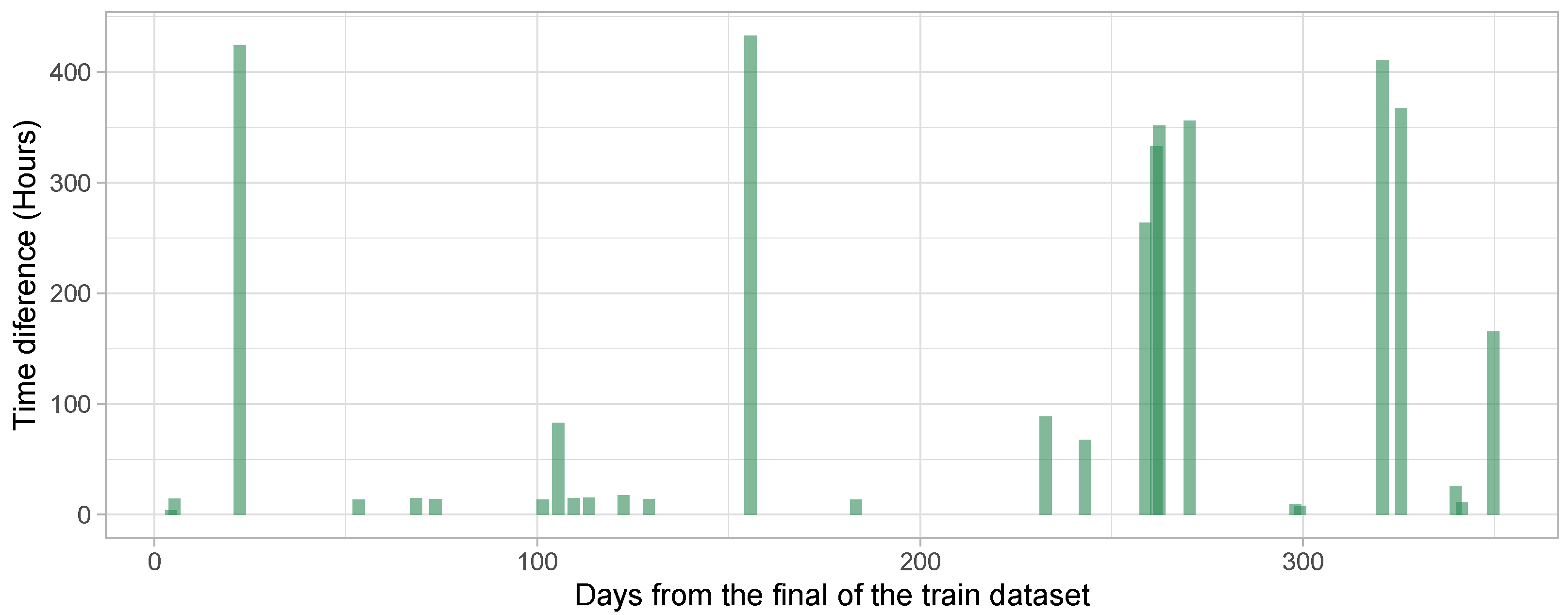
A total of 27 EQ can be recognized from the test data set, each EQ event is composed of a set of at least 15 consecutive “1” values. The middle point of each consecutive segment has been chosen to evaluate the behavior of these EQ events.

In Figure 7, the minimum time difference between the prediction of the EQ event and all the expected ones can be seen. The 50 h can be considered a reasonable limit in which it can be ensured that the prediction does not match with any EQ expected event. The time difference distribution performs substantially better when the values are close to the training data set; however, when it comes to a far distant SR, the register is not able to predict with the same level of accuracy.

The correlation between time difference and intensity of the EQ event is worth mentioning because it means that the proposed DL methodology is effectively learning to detect EQ events with lower error values when the EQ event is more powerful. In Figure 8, the correlation between the time difference and the magnitude or distance for the EQ events with less than 50 h of time difference can be observed. It is interesting to notice that EQ events with lower magnitude values are detected with more delay than higher values, contrary to our suppositions. On the other hand, the relation between time difference and distance follows our expectation. The prediction of closer EQ events is produced sooner than for the more distant ones.

Finally, a comparison without using the DL encoder was performed for validation purposes. In

Table 3. Summary of result for training and test data sets using the LSTM with the raw SR registers.

	Train Data Set	Test Data Set
Accuracy	0.5031	0.645
Sensitivity	0.07941	0.08230
Specificity	0.94543	0.91576
Pos Pred Value	0.61299	0.31974
Balanced Accuracy	0.51342	0.49903

, the results are summarized. It can be seen that the LSTM methodology is not enough to detect EQ events using SR signals. The balanced accuracy is even worse than the pure random option.

4. Conclusions

Our work led us to conclude that the usage of DL for processing SR and for exploring their relationship with other phenomena is more than promising. We have managed to develop a novel methodology for studying the SR signal based on two aspects: the dimension reduction using VAE and the study of the SR variation with a recurrent neural network (RNN) network.

These results have gone some way towards enhancing our understanding of the relationship between EQ events and the variation of the SR signal. This work has highlighted that the codification of the SR using VAE extracts valuable information at least for detecting changes in the SR pattern. Contrary to most of the literature, in this study, we have used the central peak frequency of each of the first six SR modes, which could help find these unexpected results. Our investigation into this area is still ongoing and seems likely to confirm our hypothesis; however, due to the lack of data from other observatories to compare, this finding might not be generalized to other SR registers. To further our research, we are planning to use the information from the two sensors of our observatory and also obtain SR data from observatories that were substantially distant from the Sierra de Los Filabres one, so as to enhance the accuracy of our prediction. We will also have to construct new DL architectures in order to improve the characteristics of our EQ detector models, such as temporal convolutional network (TCN) or temporal fusion transformer (TFT).