An Open Source and Reproducible Implementation of LSTM and GRU Networks for Time Series Forecasting ^†

Abstract

This paper introduces an open source and reproducible implementation of Long Short-Term Memory (LSTM) and Gated Recurrent Unit (GRU) networks for time series forecasting. We evaluated LSTM and GRU networks because of their performance reported in related work. We describe our method and its results on two datasets. The first dataset is the S&P BSE BANKEX, composed of stock time series (closing prices) of ten financial institutions. The second dataset, called Activities, comprises ten synthetic time series resembling weekly activities with five days of high activity and two days of low activity. We report Root Mean Squared Error ($RMSE$) between actual and predicted values, as well as Directional Accuracy ($DA$). We show that a single time series from a dataset can be used to adequately train the networks if the sequences in the dataset contain patterns that repeat, even with certain variation, and are properly processed. For 1-step ahead and 20-step ahead forecasts, LSTM and GRU networks significantly outperform a baseline on the Activities dataset. The baseline simply repeats the last available value. On the stock market dataset, the networks perform just as the baseline, possibly due to the nature of these series. We release the datasets used as well as the implementation with all experiments performed to enable future comparisons and to make our research reproducible.

1. Introduction

Artificial Neural Networks (ANNs) and particularly Recurrent Neural Networks (RNNs) gained attention in time series forecasting due to their capacity to model dependencies over time [1]. With our proposed method, we show that RNNs can be successfully trained with a single time series to deliver forecasts for unseen time series in a dataset containing patterns that repeat, even with certain variation; therefore, once a network is properly trained, it can be used to forecast other series in the dataset if adequately prepared.

LSTM [2] and GRU [3] are two related deep learning architectures from the RNN family. LSTM consists of a memory cell that regulates its flow of information thanks to its non-linear gating units, known as the input, forget and output gates, and activation functions [4]. GRU architecture consists of reset and update gates and activation functions. Both architectures are known to perform equally well on sequence modeling problems, yet GRU was found to train faster than LSTM on music and speech applications [5].

Empirical studies on financial time series data reported that LSTM outperformed Autoregressive Integrated Moving Average (ARIMA) [6]. ARIMA [7] is a traditional forecasting method that integrates autoregression with moving average processes. In [6], LSTM and ARIMA were evaluated on $RMSE$ between actual and predicted values on financial data. The authors suggested that the superiority of LSTM over ARIMA was thanks to gradient descent optimization [6]. A systematic study compared different ANNs architectures for stock market forecasting [8]. More specifically, the authors evaluated architectures of the types LSTM, GRU, Convolutional Neural Networks (CNN) and Extreme Learning Machines (ELM). In their experiments, two-layered LSTM and two-layered GRU networks delivered low $RMSE$.

In this study, we evaluate LSTM and GRU architectures because of their performance reported in related work for time series forecasting [6,8]. Our method is described in Section 2. In Section 2.1, Section 2.2 and Section 2.3, we review principles of Recurrent Neural Networks (RNN) of the type LSTM and GRU. In Section 2.4, we explain our data preparation, followed by the networks’ architecture, training (Section 2.5) and evaluation (Section 2.6). The evaluation was performed on two datasets. In Section 3.1, we describe the S&P BSE-BANKEX or simply BANKEX dataset, which was originally described in [8] and consists of stock time series (closing prices). In Section 3.2, we describe the Activities dataset, a dataset composed of synthetic time series resembling weekly activities with five days of high activity and two days of low activity. The experiments are presented in Section 3. Finally, we state our conclusions in Section 5 and present possible directions for future work. We release the datasets used as well as the implementation with all experiments performed to enable future comparisons and make our research reproducible.

2. Method

The general overview of the method is described as follows. The method inputs time series of values over time and outputs predictions. Every time series in the dataset is normalized. Then, the number of test samples is defined to create the training and testing sets. One time series from the train set is selected and prepared to train an LSTM and a GRU, independently. Once the networks are trained, the test set is used to evaluate $RMSE$ and $DA$ between actual and predicted values for each network. The series are transformed back to unnormalized values for visual inspection. We describe every step in detail. Next, in Section 2.1, Section 2.2 and Section 2.3, we review principles of RNNs of the type LSTM and GRU, following the presentation as in [5].

2.1. Recurrent Neural Networks

ANNs are trained to approximate a function and learn the networks’ parameters that best approximate that function. RNNs are a special type of ANNs developed to handle sequences. An RNN updates its recurrent hidden state $h_t$ for a sequence $x=(x_1,x_2,\dots ,x_T)$ by:

$$h_t=\left\{\begin{array}{cc}0,& t=0\\ \varphi (h_{t-1},x_t),& otherwise,\end{array}\right.$$

(1)

where $\varphi$ is a nonlinear function. The output of an RNN maybe of variable length $y=(y_1,y_2,\dots ,y_T)$.

The update of $h_t$ is computed by:

$$h_t=g(W{x}_t+U{h}_{t-1}),$$

(2)

where W and U are weights’ matrices and g is a smooth and bounded activation function such as a logistic sigmoid, or simply called sigmoid function $f\left(x\right)=\sigma =\frac{1}{1+e^{-x}}$, or a hyperbolic tangent function $f\left(x\right)=tanh\left(x\right)=\frac{e^x-e^{-x}}{e^x+e^{-x}}$.

Given a state $h_t$, an RNN outputs a probability distribution for the next element in a sequence. The sequence probability is represented as:

$$p(x_1,x_2,\dots ,x_T)=p\left(x_1\right)p(x_2\mid x_1)\dots p(x_T\mid x_1,x_2,\dots ,x_{T-1}).$$

(3)

The last element is a so-called end-of-sequence value. The conditional probability distribution is given by:

$$p(x_t\mid x_1,x_2,\dots x_{t-1})=g\left(h_t\right),$$

(4)

where $h_t$ is the recurrent hidden state of the RNN as in expression (1). Updating the network’s weights involves several matrix computations, such that back-propagating errors lead to vanishing or exploding weights, making training unfeasible. LSTM was proposed in 1997 to solve this problem by enforcing constant error flow thanks to gating units [2]. GRU is a closely related network proposed in 2014 [3]. Next, we review LSTM and GRU networks. See Figure 1 for illustration.

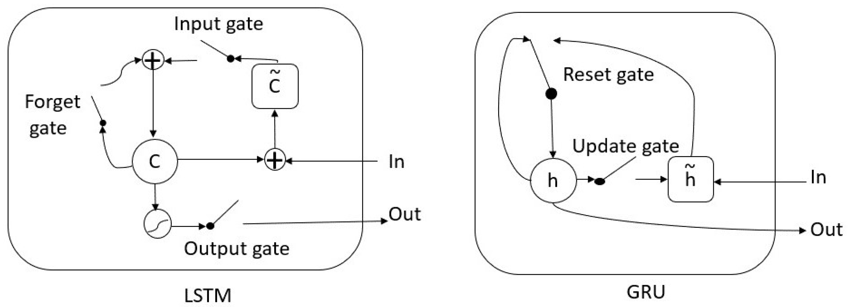
2.2. Long Short-Term Memory

The LSTM unit decides whether to keep content memory thanks to its gates. If a sequence feature is detected to be relevant, the LSTM unit keeps track of it over time, modeling dependencies over long-distance [5].

In Expressions (6)–(8) and (10), W and U represent weights matrices and V represents a diagonal matrix. W, U and V need to be learned by the algorithm during training. The subscripts i, o and f correspond to input, output and forget gates, respectively. For every j-th LSTM unit, there is a memory cell $c_t^j$ at time t, which activation $h_t^j$ is computed as:

$$h_t^j=o_t^{j}tanh\left(c_t^j\right)$$

(5)

where $o_t^j$ is the output gate responsible for modulating the amount of memory in the cell. The forget gate $f_t^j$ modulates the amount of memory content to be forgotten and the input gate $i_t^j$ modulates the amount of new memory to be added to the memory cell, such that:

$$o_t^j=\sigma {(W_o{x}_t+U_o{h}_{t-1}+V_o{c}_t)}^j,$$

(6)

$$f_t^j=\sigma {(W_f{x}_t+U_f{h}_{t-1}+V_f{c}_{t-1})}^j,$$

(7)

$$i_t^j=\sigma {(W_i{x}_t+U_i{h}_{t-1}+V_i{c}_{t-1})}^j.$$

(8)

where $\sigma$ is a sigmoid function. The memory cell $c_t^j$ partially forgets and adds new memory content ${\tilde{c}}_t^j$ by:

$$c_t^j=f_t^j{c}_{t-1}^j+i_t^j{\tilde{c}}_t^j,$$

(9)

where:

$${\tilde{c}}_t^j=tanh{(W_c{x}_t+U_c{h}_{t-1})}^j.$$

(10)

2.3. Gated Recurrent Unit

The main difference between LSTM and GRU is that GRU does not have a separate memory cell, such that the activation $h_t^j$ is obtained by the following expression:

$$h_t^j=(1-z_t^j)h_{t-1}^j+z_t^j{\tilde{h}}_t^j.$$

(11)

The update gate $z_t^j$ decides the amount of update content given by the previous $h_{t-1}^j$ and candidate activation ${\tilde{h}}_t^j$. In Expressions (12)–(14), W and U represent weights matrices that need to be learned during training. Moreover, the subscripts z and r correspond to update and reset gates, respectively. The update gate $z_t^j$ and reset gate $r_t^j$ are obtained by the following expressions:

$$z_t^j=\sigma {(W_z{x}_t+U_z{h}_{t-1})}^j,$$

(12)

$$r_t^j=\sigma {(W_r{x}_t+U_r{h}_{t-1})}^j,$$

(13)

where $\sigma$ is a sigmoid function. The candidate activation ${\tilde{h}}_t^j$ is obtained by:

$${\tilde{h}}_t^j=tanh{(W{x}_t+r_t\odot \left(U{h}_{t-1}\right))}^j.$$

(14)

where ⊙ denotes element-wise multiplication.

2.4. Data Preparation

Every time series or sequence in the dataset is normalized as follows. Let v be a sequence $v=(v_1,v_2,\dots ,v_Q)$ of Q samples that can be normalized between 0 and 1:

$$x=v^{\prime }=\frac{v-v_{min}}{v_{max}-v_{min}}.$$

(15)

We define the number of samples in the test set as $tes{t}_s$. The number of samples N for training is obtained by $N=Q-tes{t}_s-w$. Then, a sequence x is selected arbitrarily and prepared to train each network as follows. We define a window of size w and a number of steps ahead f, where $f<w<N<Q$, such that:

$$X=\left[\begin{array}{cccc}{x}_1& x_2& \dots & x_w\\ x_2& x_3& \dots & x_{w+1}\\ x_3& x_4& \dots & x_{w+2}\\ \dots & \dots & \dots & \dots \\ x_{Q-(w-1+f)}& x_{Q-(w-2+f)}& \dots & x_{Q-f}\end{array}\right],$$

X becomes a $Q-(w-1+f)$ by w matrix, and:

$$Y=\left[\begin{array}{cccc}{x}_{w+1}& x_{w+2}& \dots & x_{w+f}\\ x_{w+2}& x_{w+3}& \dots & x_{w+2+f}\\ x_{w+3}& x_{w+4}& \dots & x_{w+3+f}\\ \dots & \dots & \dots & \dots \\ x_{Q-(f-1)}& x_{Q-(f-2)}& \dots & x_Q\end{array}\right]$$

(16)

becomes a $Q-(w-1+f)$ by f matrix containing the targets. The first N rows of X and Y are used for training. The remaining $Q-N$ elements are used for testing. The settings for our experiments are described in Section 3, after we introduce the characteristics of the dataset used.

2.5. Networks’ Architecture and Training

We tested two RNNs. One with LSTM memory cells and one with GRU memory cells. In both cases, we use the following architecture and training:

• A layer with 128 units,
• A dense layer with size equal to the number of steps ahead for prediction,

With recurrent sigmoid activations and $tanh$ activation functions as explained in Section 2.2 and Section 2.3. The networks are trained for 200 epochs with Adam optimizer [9]. The number of epochs and architecture were set empirically. We minimize Mean Squared Error ($MSE$) loss between the targets and the predicted values, see Expression (17). The networks are trained using a single time series prepared as described in Section 2.4. The data partition is explained in Section 3.3.

2.6. Evaluation

We use Mean Squared Error ($MSE$) to train the networks:

$$MSE=n^{-1}\sum _{t=1}^n{(x_t-y_t)}^2,$$

(17)

where n is the number of samples, $x_t$ and $y_t$ are actual and predicted values at time t. Moreover, we use Root Mean Squared Error ($RMSE$) for evaluation between algorithms:

$$RMSE=\sqrt{MSE}.$$

(18)

Both metrics, $MSE$ and $RMSE$, are used to measure the difference between actual and predicted values, and therefore, smaller results are preferred [10]. We also use Directional Accuracy ($DA$):

$$DA=\frac{100}{n}\sum _{t=1}^n{d}_t,$$

(19)

where:

$$d_t=\left\{\begin{array}{cc}1& (x_t-x_{t-1})(y_t-y_{t-1})\ge 0\\ 0& otherwise.\end{array}\right.$$

such that $x_t$ and $y_t$ are the actual and predicted values at time t, respectively, and n is the sample size. $DA$ is used to measure the capacity of a model to predict direction as well as prediction accuracy. Thus, higher values of $DA$ are preferred [10].

3. Experiments

In this section, we report experiments performed with both datasets.

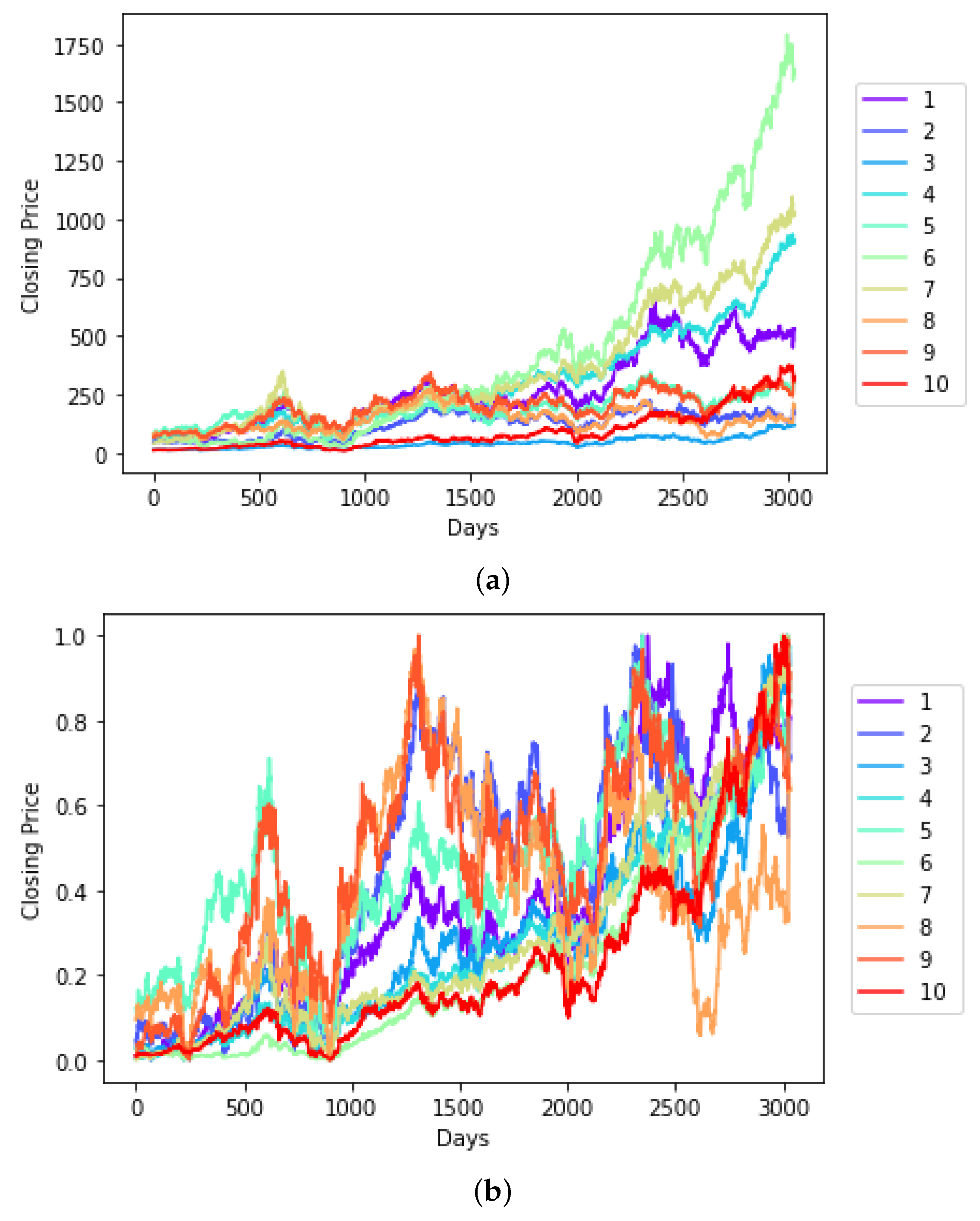
3.1. The S&P BSE BANKEX Dataset

This dataset was originally described in [8]; however, our query retrieved a different number of samples as in [8]. We assume it must have changed since it was originally retrieved. We collected the time series on 20 January 2022, using Yahoo! Finance’s API [11] for the time frame between 12 July 2005, and 3 November 2017, see

Table 1. Entities in the S&P BSE-BANKEX Dataset.

Number	Entity	Symbol
1	Axis Bank	AXISBANK.BO
2	Bank of Baroda	BANKBARODA.BO
3	Federal Bank	FEDERALBNK.BO
4	HDFC Bank	HDFCBANK.BO
5	ICICI Bank	ICICIBANK.BO
6	Indus Ind Bank	INDUSINDBK.BO
7	Kotak Mahindra	KOTAKBANK.BO
8	PNB	PNB.BO
9	SBI	SBIN.BO
10	Yes Bank	YESBANK.BO

. Most time series had 3035 samples, and some time series had 3032 samples; therefore, we stored each time series’s last 3032 samples. Figure 2 presents the time series of BANKEX without and with normalization.

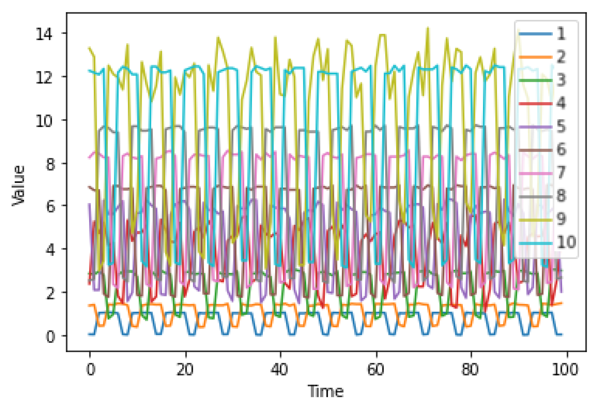
3.2. The Activities Dataset

The Activities dataset is a synthetic dataset created resembling weekly activities with five days of high activity and two days of low activity. The dataset has ten time series with 3584 samples per series. Initially, a pattern of five ones followed by two zeros was repeated to obtain a length of 3584 samples. The series was added a slope of $0.0001$. The original series was circularly rotated for the remaining series in the dataset, to which noise was added, and each sequence was arbitrarily scaled, so that the peak-to-peak amplitude of each series was different, see Figure 3.

3.3. Datasets Preparation and Partition

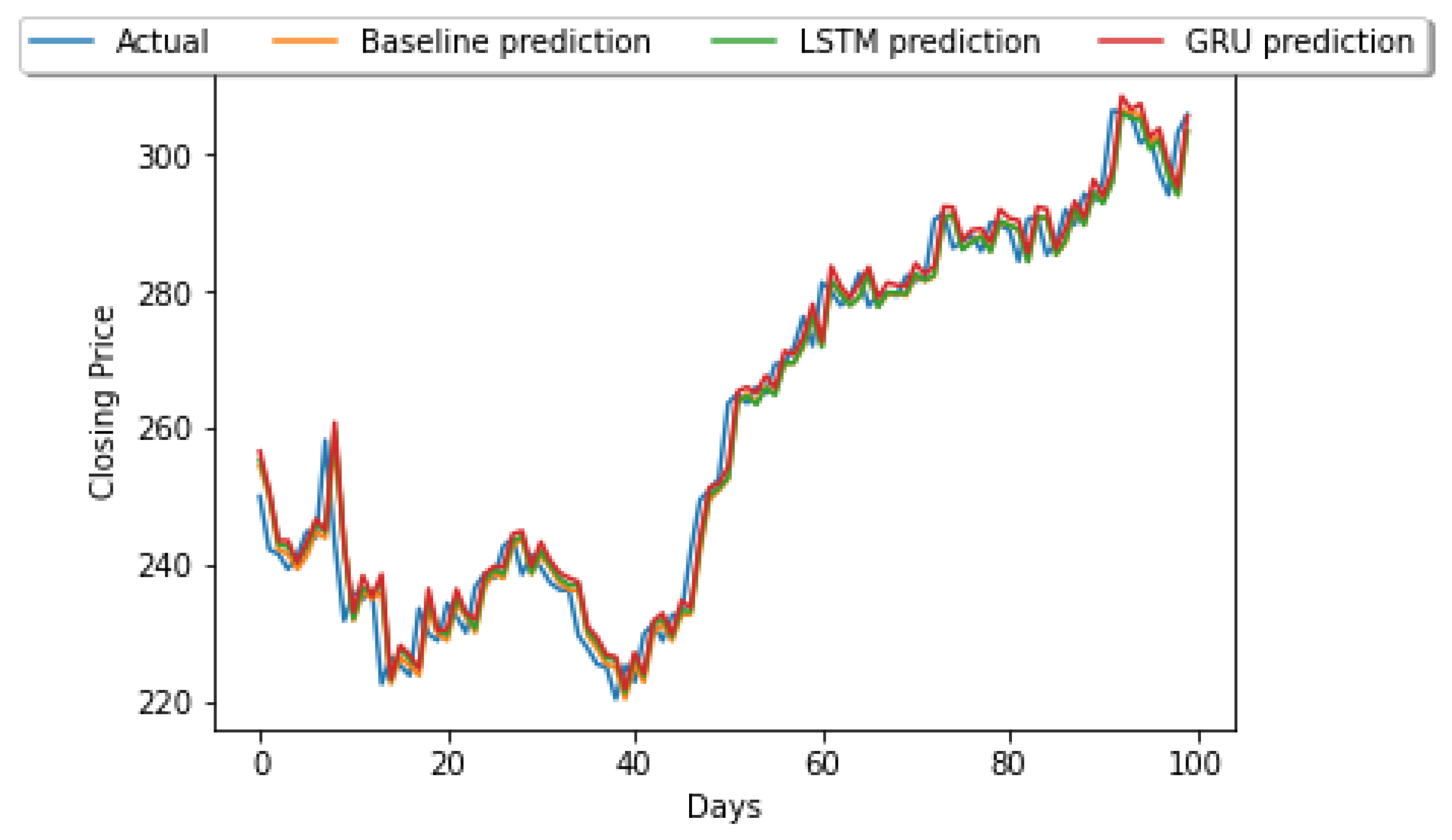
Following Section 2.4, every time series was normalized between 0 and 1. We used a window of size $w=60$ days. We tested for $f=1$ and $f=20$ steps ahead. We used the last 251 samples of each time series for testing. We selected arbitrarily the first time series of each dataset for training our LSTM and GRU networks.

3.4. Results

The results are presented in

Table 2. One-step ahead forecast on Activities dataset. RMSE: columns 2 to 4. DA: columns 5 to 7.

	RMSE			DA
	LSTM	GRU	Baseline	LSTM	GRU	Baseline
Mean	0.2949	0.1268	0.3730	0.6360	0.6236	0.4212
SD	0.0941	0.0425	0.0534	0.0455	0.0377	0.0403

,

Table 3. Twenty-step ahead forecast on Activities dataset. RMSE: columns 2 to 4. DA: columns 5 to 7.

	RMSE			DA
	LSTM	GRU	Baseline	LSTM	GRU	Baseline
Mean	0.1267	0.2048	0.4551	0.6419	0.6261	0.4805
SD	0.0435	0.0683	0.0678	0.0331	0.0255	0.0413

,

Table 4. One-step ahead forecast on BANKEX dataset. RMSE: columns 2 to 4. DA: columns 5 to 7.

	RMSE			DA
	LSTM	GRU	Baseline	LSTM	GRU	Baseline
Mean	0.0163	0.0163	0.0161	0.4884	0.4860	0.4880
SD	0.0052	0.0056	0.0056	0.0398	0.0385	0.0432

and

Table 5. Twenty-step ahead forecast on BANKEX dataset. RMSE: columns 2 to 4. DA: columns 5 to 7.

	RMSE			DA
	LSTM	GRU	Baseline	LSTM	GRU	Baseline
Mean	0.0543	0.0501	0.0427	0.5004	0.5004	0.4969
SD	0.0093	0.0064	0.0113	0.0071	0.0087	0.0076

. Close-to-zero $RMSE$ and close-to-one $DA$ are preferred. On the Activities dataset, two-tailed Mann–Whitney tests show that for 1-step ahead forecasts, $RMSE$ achieved by any RNN is significantly lower than that delivered by the baseline (LSTM & Baseline: $U=19,n=10,10,p<0.05$. GRU & Baseline: $U=0,n=10,10,p<0.05$). In addition, GRU delivers significantly lower $RMSE$ than LSTM ($U=91,n=10,10,p<0.05$). In terms of $DA$, both RNN perform equally well and significantly outperform the baseline. For 20-step ahead forecasts, again both RNNs achieve significantly lower $RMSE$ than the baseline (LSTM & Baseline: $U=0,n=10,10,p<0.05$. GRU & Baseline: $U=0,n=10,10,p<0.05$). This time, LSTM achieves lower $RMSE$ than GRU ($U=10,n=10,10,p<0.05$) and higher $DA$ ($U=81,n=10,10,p<0.05$).

On the BANKEX dataset, two-tailed Mann–Whitney tests show that for 1-step ahead forecasts there is no difference among approaches considering $RMSE$ (LSTM & Baseline: $U=51,n=10,10,p>0.05$. GRU & Baseline: $U=55,n=10,10,p>0.05$. LSTM & GRU: $U=49,n=10,10,p>0.05$). Similar results are found for 20-step ahead forecasts (LSTM & Baseline: $U=76,n=10,10,p>0.05$. GRU & Baseline: $U=67,n=10,10,p>0.05$. LSTM & GRU: $U=66,n=10,10,p>0.05$). $DA$ results are consistent with those obtained for $RMSE$. Figure 4a,b show examples of 20-step ahead forecasts and Figure 5 presents an example of 1-step ahead forecasts. Visual inspection helps understand the results.

4. Discussion

The motivation for developing a reproducible and open-source framework for time series forecasting relates to our experience in trying to reproduce previous work [6,8]. We found it challenging to find implementations that are simple to understand and replicate. In addition, datasets are not available. We discontinued comparisons with [8], since the dataset we collected was slightly different, and we were unsure if the reported results referred to normalized values or not. If the algorithms are described but the implementations are not available, a dataset is necessary to compare forecasting performance between two algorithms, such that a statistical test can help determine if one algorithm is significantly more accurate than the other [12] (pp. 580–581).

5. Conclusions

We proposed a method for time series forecasting based on LSTM and GRU and showed that these networks can be successfully trained with a single time series to deliver forecasts for unseen time series in a dataset containing patterns that repeat, even with certain variation. Once a network is properly trained, it can be used to forecast other series in the dataset if adequately prepared. We tried and varied several hyperparameters. On sequences, such as those resembling weekly activities that repeat with certain variation, we found an appropriate setting; however, we failed to find an architecture that would outperform a baseline on stock market data; therefore, we assume that we either failed at optimizing the hyperparameters of the networks, the approach is unsuitable for this application, or we would need extra information that is not reflected in stock market series alone. For future work, we plan to benchmark different forecasting methods against the method presented here. In particular, we want to evaluate statistical methods as well as other machine learning methods that have demonstrated strong performance on forecasting tasks [13]. We release our code as well as the dataset used in this study to allow this research to be reproducible.

References

1. Rumelhart, D.E.; Hinton, G.E.; Williams, R.J. Learning representations by back-propagating errors. Nature 1986, 323, 533–536. [Google Scholar] [CrossRef]
2. Hochreiter, S.; Schmidhuber, J. Long short-term memory. Neural Comput. 1997, 9, 1735–1780. [Google Scholar] [CrossRef] [PubMed]
3. Cho, K.; Van Merriënboer, B.; Bahdanau, D.; Bengio, Y. On the properties of neural machine translation: Encoder-decoder approaches. arXiv 2014, arXiv:1409.1259. [Google Scholar]
4. Greff, K.; Srivastava, R.K.; Koutník, J.; Steunebrink, B.R.; Schmidhuber, J. LSTM: A search space odyssey. IEEE Trans. Neural Netw. Learn. Syst. 2016, 28, 2222–2232. [Google Scholar] [CrossRef] [PubMed] [Green Version]
5. Chung, J.; Gulcehre, C.; Cho, K.; Bengio, Y. Empirical evaluation of gated recurrent neural networks on sequence modeling. arXiv 2014, arXiv:1412.3555. [Google Scholar]
6. Siami-Namini, S.; Tavakoli, N.; Namin, A.S. A comparison of ARIMA and LSTM in forecasting time series. In Proceedings of the 2018 17th IEEE International Conference on Machine Learning and Applications (ICMLA), Orlando, FL, USA, 17–20 December 2018; pp. 1394–1401. [Google Scholar]
7. Box, G.; Jenkins, G. Time Series Analysis: Forecasting and Control; Holden-Day: San Francisco, CA, USA, 1970. [Google Scholar]
8. Balaji, A.J.; Ram, D.H.; Nair, B.B. Applicability of deep learning models for stock price forecasting an empirical study on BANKEX data. Procedia Comput. Sci. 2018, 143, 947–953. [Google Scholar] [CrossRef]
9. Kingma, D.P.; Ba, J. Adam: A method for stochastic optimization. arXiv 2014, arXiv:1412.6980. [Google Scholar]
10. Wang, J.J.; Wang, J.Z.; Zhang, Z.G.; Guo, S.P. Stock index forecasting based on a hybrid model. Omega 2012, 40, 758–766. [Google Scholar] [CrossRef]
11. Yahoo. Yahoo! Finance’s API. 2022. Available online: https://pypi.org/project/yfinance/ (accessed on 20 January 2022).
12. Alpaydin, E. Introduction to Machine Learning; The MIT Press: Cambridge, MA, USA; London, UK, 2014. [Google Scholar]
13. Makridakis, S.; Spiliotis, E.; Assimakopoulos, V. M5 accuracy competition: Results, findings, and conclusions. Int. J. Forecast. 2022. [Google Scholar] [CrossRef]
Figure 1. LSTM (left) and GRU (right). c represents the memory cell and c ˜ the new memory cell of the LSTM. h represents the activation and h ˜ the new activation of the GRU. Based on [5].
Engproc 18 00030 g001
Figure 2. (a) Time series in the BANKEX dataset without normalization. Closing Price in Indian Rupee (INR). Daily samples retrieved between 12 July 2005 and 3 November 2017 using Yahoo! Finance’s API [11]. All time series with 3032 samples. (b) Same time series as in (a), but with normalization; closing price normalized between 0 and 1. The numbers from 1 to 10 correspond to the numbers (first column) for each series in Table 1.
Engproc 18 00030 g002
Figure 3. Time series in the Activities dataset without normalization, first 100 samples.
Engproc 18 00030 g003
Figure 4. Examples of 20-step ahead forecast. (a) Activities dataset. (b) BANKEX dataset.
Engproc 18 00030 g004
Figure 5. Example of 1-step ahead forecast. Actual and predicted closing price over the first 100 days of the test set Yes Bank. Closing Price in Indian Rupee (INR).
Engproc 18 00030 g005