Combination of Post-Processing Methods to Improve High-Resolution NWP Solar Irradiance Forecasts in French Guiana ^†

Abstract

Efforts have been made to improve Numerical Weather Prediction (NWP) forecasts using post-processing techniques, relying on statistical models to refine the weather forecasts. Most approaches used in the literature suffer from two main deficiencies when applied to high-resolution data: (1) they high capacity models to retain nonlinear data fluctuations; (2) some are known to reduce the mean random error; however, they may still generate subsequent biased forecasts. In this study, methods from three different approaches are compared to improve 10-min resolution NWP solar irradiance forecasts, namely a neural network and a linear statistical model as Model Output Statistics, Kalman Filter and Kernel Conditional Density Estimation. The results show that none of the methods, if used individually, improve the mean absolute error (MAE) and mean bias (MBE) jointly. However, a combination of a neural network followed by Kalman filter post-processing results in significant improvements both in the mean random error and the systematic mean bias of original forecasts, reducing the MAE by 45% and the MBE by 91%, respectively.

1. Introduction

The accurate forecasting of solar irradiance plays an essential role in the management and integration of photovoltaic (PV) systems in transmission grids. The intermittence of solar irradiance, which is highly correlated with the output power, needs to be accurately predicted in advance. It assures the transport system operator that sufficient power will be available to fill the demand throughout the day.

Numerical weather prediction (NWP) models have been widely utilized to generate medium and long-term forecasts of solar irradiance, relying on mathematical equations describing the atmospheric fluid mechanics and thermodynamics [1]. Admittedly, NWP modeling has improved continuously; however, the resulting weather forecasts often present considerable errors. These errors can be divided into two groups: random errors, caused by the insufficient capacity of NWP models to predict the variations of solar irradiance, and systematic bias, caused by defective modeling which will tend to systematically overestimate or underestimate solar irradiance.

Over the past decades, different post-processing techniques were proposed to correct these deviations. Most of the proposed methods follow the approach called model output statistics (MOS) [2,3,4,5], where NWP forecast errors are corrected by learning a function that relates the response variable of interest to its predictors. Despite improving the performance of the original forecasts, the approach suffers from two primary deficiencies if applied to high-resolution data: (1) it requires a model with a high capacity to retain nonlinear data fluctuations; (2) it is known to reduce the random error; however, it may still generate subsequent biased forecasts.

Besides MOS, other approaches have also been used in the literature for the same purpose, without sharing the same drawbacks: the Kalman filter (KF) [6,7,8,9,10,11] recursively improves weather forecasts based on historical errors measured before the forecast generation, and Kernel Conditional Density Estimation (KCDE) [1] allows estimations of the marginal distribution of original forecasts–and consequently, their expected value–conditioned on other explanatory variables.

The objective of this study is to fill the gap in the post-processing of high-resolution forecasts observed in the literature by proposing a global approach to enhance solar irradiance forecasts based on the consecutive combination of post-processing methods, which do not effectively enhance the global performance of the original forecasts when applied individually. Furthermore, the same analysis is proposed for coarser forecasts, revealing differences in the modeling and efficiency of post-processing methods based on temporal resolution.

2. Methodology

The methods to be compared and combined are introduced in this section, namely the MOS, KCDE, and Kalman filters.

2.1. Model Output Statistics

MOS are statistical models that relate observed variables of interest (prediction error, in this case) with the appropriate predictors derived from the outputs of the original model (original NWP predictions). Once calibrated, MOS models are used to estimate the prediction error of WRF forecasts, which are then subtracted from original forecasts, thereby generating improved forecasts. An artificial neural network (ANN) is selected from MOS methods, which are proven to provide better improvements for high-resolution data. A statistical MOS was selected for an additional comparison.

2.1.1. Artificial Neural Network

In ANNs, the function parameters are processing units, called neurons. They are interconnected via a set of weights-analogous to synaptic connections in the nervous system in a manner that allows signals to travel through the network when making predictions or during training. The neurons are grouped in consecutive layers, where each layer is responsible to model patterns of different complexity levels. In this study, a multi-layer perceptron is used as a neural network, where each neuron of one layer is connected to every neuron of the following layer. The output of any neuron is equal to the sum of the outputs of all neurons of the previous layer multiplied by their respective weights, plus a bias term. Subsequently, the net output is passed to an activation function that bounds the activation value to a predefined range. The activation function employed is known as a rectified linear unit (ReLU), which helps the convergence of the model and presents good results. Finally, the model output is equal to the activation value of the only neuron in the output layer.

During training, the weights and biases are updated to reduce the mean square error for each batch of predictions and observations, using the Adam stochastic gradient descent. This process is repeated multiple times, called epochs, that covers the training dataset extensively until the maximum number of epochs is reached.

2.1.2. Lorenz’s MOS

As compared to the neural networks, the success of Lorenz’s MOS [12] can be partly attributed to its simplicity. In particular, the error was first modeled as a 4th-order polynomial function:

$$e=a_1{cos}^{4}Z+a_2{\widehat{k}}^4+a_3{cos}^{3}Z+...+a_8\widehat{k}$$

(1)

where e defines the error between the forecasted and measured solar irradiance. The model presented by Lorenz relies on two predictors: Z defining the zenith angle and $\widehat{k}$ for the forecasted clear-sky index–the ratio of solar irradiance forecasts to the expected solar irradiance in clear-sky conditions.

The function parameters can be easily estimated using the least squared method over historical forecasts and measurements. Similar to all tested methods, the best group of predictors was selected based on their capability of predicting the original forecast error.

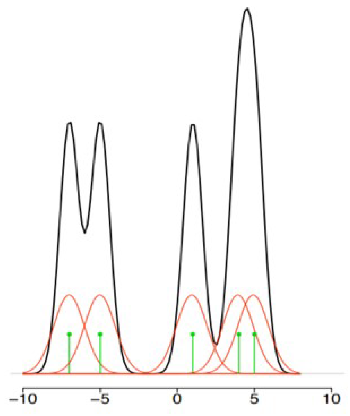
2.2. Kernel Conditional Density Estimation

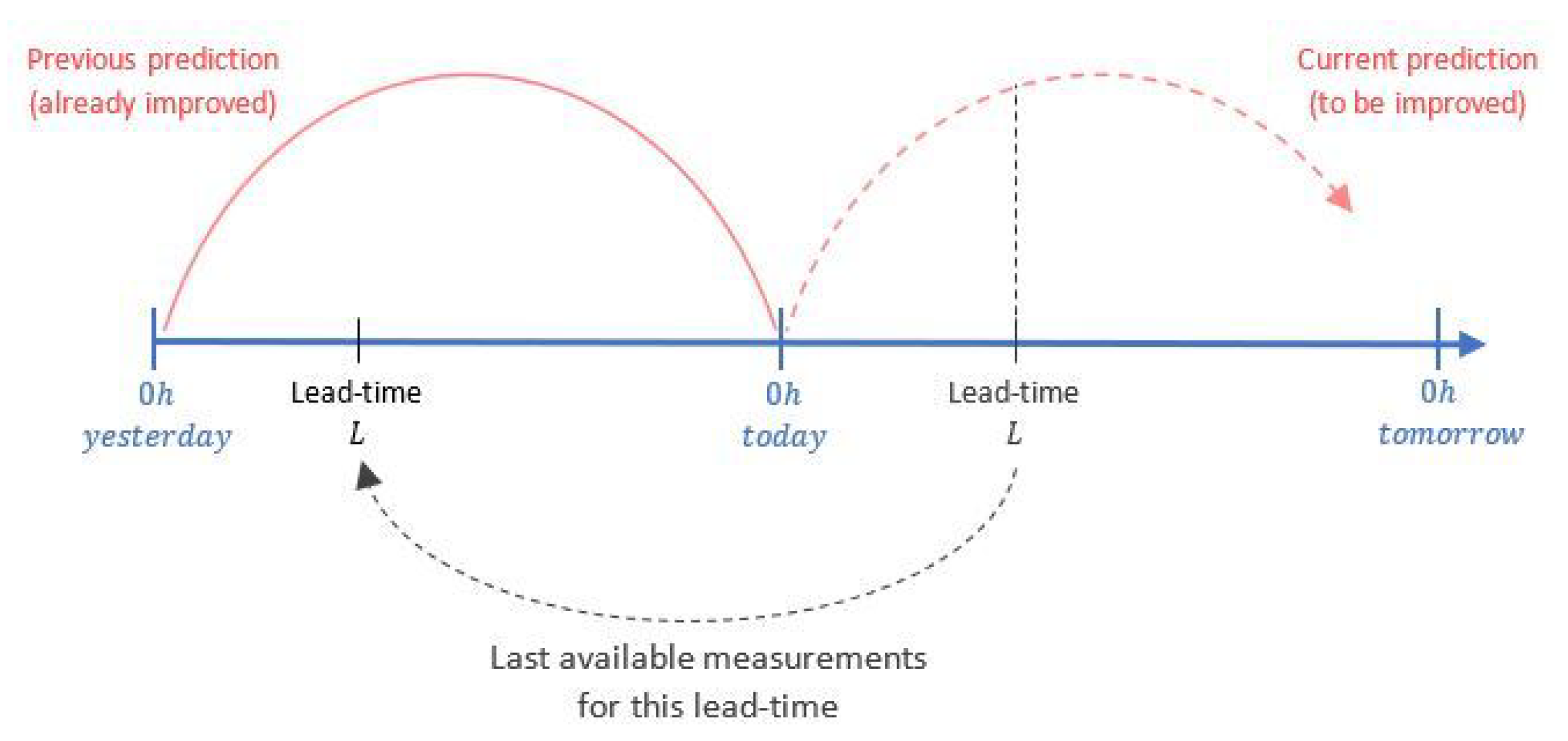
Kernel density estimation is a probabilistic nonparametric approach for estimating the unknown distribution of a random variable x (e.g., the original forecast error), based on the local estimation of the distribution of its samples X₁, …, X_n [1], as shown in Figure 1.

The kernel, referring to any smooth function K, is used to define the distributions assigned to each sample x, which will then compose the estimated probability function. The most used kernel is the Gaussian kernel, which is defined by:

$$\mathcal{K}\left(x\right)=\frac{1}{\sqrt{2\pi }}{e}^{-\frac{x^2}{2}}$$

(2)

It is equivalent to the probability density function of a standard normal distribution. A scaled version allows to handle variables varying in different ranges:

$${\mathcal{K}}_h\left(x\right)=\frac{1}{h}\mathcal{K}\left(\frac{x}{h}\right)$$

(3)

where h denotes the bandwith parameter controlling the smoothness of the density estimates. For the density estimation of a dataset presenting n values, the kernel density estimator is defined as follows:

$$\widehat{f}\left(x\right)=\sum _{n=1}^n\frac{1}{n}\mathcal{K}(x-X_i)$$

(4)

Ultimately, the conditional version of this density estimation adds a weighting factor proportional to the magnitude of each value along one dimension:

$$\widehat{f}\left(y\right|x)=\sum _{n=1}^n{w}_i\left(x\right){\mathcal{K}}_{h_y}(y-Y_i)$$

(5)

where

$$w_i\left(x\right)=\frac{{\mathcal{K}}_{h_x}\left(∥x-X_i∥\right)}{{\sum }_{n=1}^n{\mathcal{K}}_{h_x}\left(∥x-X_i∥\right)}$$

(6)

Interested readers are invited to read the comprehensive definition of the KCDE method provided by Yang [1].

Different methods have been proposed to find the optimal value of the bandwidths h_x and h_y. In this study, a method described in [1] was employed, where the selected bandwidth is the one that minimizes the asymptotic mean integrated squared error (AMISE). For circular data presenting a periodic nature, such as the solar zenith angle, a different kernel is proposed, called the von Mises kernel, which requires adaptations to define an expression for the AMISE during the application of the bandwidth selection method. Finally, for one group of predictors, the point forecasts for the prediction error can be obtained by calculating the expectation of the resulting probability density function generated with the kernel conditional density estimation.

2.3. Kalman Filter

In a general presentation, Kalman filters are used to estimate the error state $x\in {\mathbb{R}}^n$ of a discrete time-evolving process. At each time step, the first-guess of the error state is as follows:

$$x_t=A{x}_{t-1}+w_t$$

(7)

where matrix A defines the values of pre-defined predictors at one time step, and the state is a vector representing the effect of each predictor when estimating the prediction error. A nonlinear Kalman filter can be implemented by adding nonlinearities to matrix A, such as predictors in the exponential form.

The observed errors $z\in {\mathbb{R}}^m$ expressed by a measurement equation that relates the error to measurements for each time step is as follows:

$$z_t=H{x}_t+v_t$$

(8)

The variable $x_{t-1}$ represents the previous error state, and random variables $w_t$ and $v_t$ are white noises applied to model perturbations in the process and measurements, respectively. The noises are assumed to be independent of each other and follow normal distributions with covariances W and V:

$$\begin{array}{cc}\hfill p\left(w\right)& \sim N(0,W)\hfill \\ \hfill p\left(v\right)& \sim N(0,V)\hfill \end{array}$$

(9)

In practice, the process noise covariance W and measurement noise covariance V matrices may change with each time step or measurement and are calculated iteratively with recent values. The same process is applied to the matrices A and H.

The correction procedure involves two groups of equations: time update equations and measurements update equations, time update equations are responsible for making a first guess of the next solar irradiance prediction error, based on the last state of the measured error and error covariance estimates, obtaining an a priori prediction for the next time step; the measurement update equations will then incorporate new measurements into the first guess, obtaining improved a posteriori predictions [13]. The interested reader is referred to [7] for a detailed description of the associated equations.

As mentioned in [1], if the Kalman filter is applied continuously for each lead-time of a day-ahead or intraday prediction, such forecast horizon becomes «resolution-ahead»; e.g, hour-ahead if working in hourly resolution. The procedure needs to be adapted when applied operationally, keeping forecasts in the original horizon. As the original forecasts are issued every day at 00:00 in this study, the first guess at a lead-time L within the horizon of 24 h cannot depend on the previous lead-time L−1 of the same forecast, because the values for the entire forecast are still first guesses, as respective measurements are not yet accessible and update equations cannot be applied. The first guess for the lead-time L should be made based on the same lead-time with available measurements, in this case, the lead-time L of the forecast already improved the day before. A scheme of this procedure is presented in Figure 2.

Unlike MOS methods, Kalman filters do not require parameters to be trained with extensive historical information. However, the method requires recurrent access to observations at each time step, therefore being more efficient in real-time applications rather to improve long-range forecasts.

3. Data

3.1. Weather Forecasts

The weather forecasts used in this study were issued daily at 00:00 by a Weather Research and Forecasting (WRF) numerical model during a year and aggregated in a 10-min resolution.

The WRF forecasts include the global horizontal irradiance to be post-processed and correlated weather variables, which are used as predictors.

Considerable errors were observed in solar irradiance WRF forecasts for low levels of sun elevation (below 15°). These errors can be explained by the approximations made to model the atmosphere within WRF, resulting in more forecast errors when the sunlight crosses larger distances in the atmosphere, like in the early morning and late afternoon. Therefore, the time steps before 8 a.m. and after 5 p.m. were removed from the analysis to avoid such outliers.

3.2. Observations

Ground truth of solar irradiance was obtained with a pyranometer installed at the same location in French Guiana to evaluate and calibrate certain post-processing methods.

The observations were preprocessed with the imputation of outliers or missing values through linear interpolation if they were less than 30% of the day, otherwise the entire day was discarded.

Besides the high-resolution forecasts and observations, a second group of data was obtained by upscaling the same data to an hourly resolution. The objective is to verify the differences in modeling and performance of each method when applying to coarse-grained and fine-grained time series. Figure 3 presents observations in both temporal resolutions for a specific day.

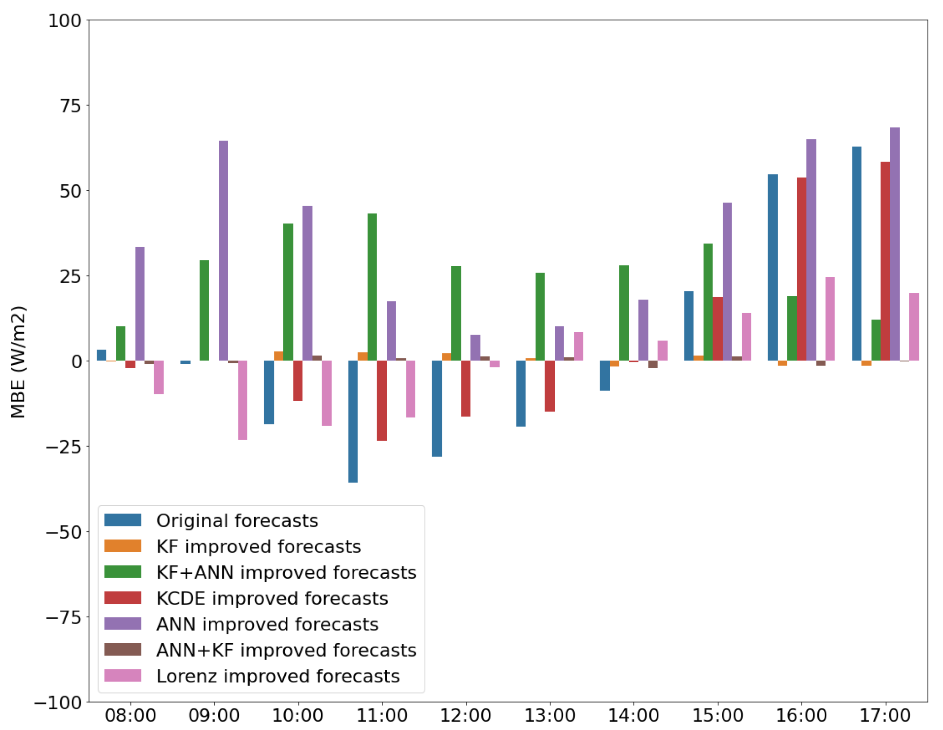
4. Results and Discussion

The methods described in the previous section and convenient combinations were applied to the post-processing of WRF solar irradiance forecasts in both 10-min resolution and hourly resolution. Accordingly, particularities in the modeling of each time-resolution forecast and obtained results are described in this section.

4.1. Modeling

Post-processing was applied for each method using different combinations of different numbers of predictors. In particular, for ANN, a second search was performed over the parameters of the model, such as the batch size, number of layers, and neurons per layer. The Kalman filter was tested in both linear and nonlinear implementations, with different combinations of exponential predictors in the latter case. The best group of predictors found for each method and for each time-resolution tested are listed in

Table 1. Optimal group of predictors per method per resolution.

Resolution	ANN	Lorenz	KCDE	Kalman Filter
10-min	$Irradianc{e}_{pred}$ Wind speed (x) Wind speed (y) Cloud-coverage Temperature Humidity	$Irradianc{e}_{pred}$ Cloud-coverage Sun zenith angle Pressure Temperature Wind speed (x)	$Irradianc{e}_{pred}$ Cloud-coverage Sun zenith angle Pressure	$Irradianc{e}_{pred}$ Cloud-coverage
Hourly	$Irradianc{e}_{pred}$ Wind speed (x) Wind speed (y) Cloud-coverage Temperature Humidity Sun zenith angle	$Irradianc{e}_{pred}$ Cloud-coverage Sun zenith angle Pressure Temperature Wind speed (x)	$Irradianc{e}_{pred}$ Cloud-coverage Sun zenith angle	$Irradianc{e}_{pred}$ Cloud-coverage

.

MOS and Kalman filter methods were implemented in python, using the Keras library for neural networks, while KCDE was implemented in R using the stats package.

The best groups of predictors used to improve higher resolutions are slightly bigger, which can be explained by the required additional data to explain more sudden variations of solar irradiance. Furthermore, the methods focusing on correcting the random error (e.g., ANN, Lorenz’s MOS) tend to require more predictors than methods that focus on the mean bias (e.g., Kalman filter).

In particular, for the Kalman filter, the historical data used in the recursive calculation of predicted bias at each time step is also a parameter to be defined. Basically, the random errors can be better modeled if the historical window is longer, and conversely, a shorter historical window allows for better mean bias modeling. After multiple tests, the optimal window length capable of reducing both the random error and mean bias is 70 days for both time resolutions.

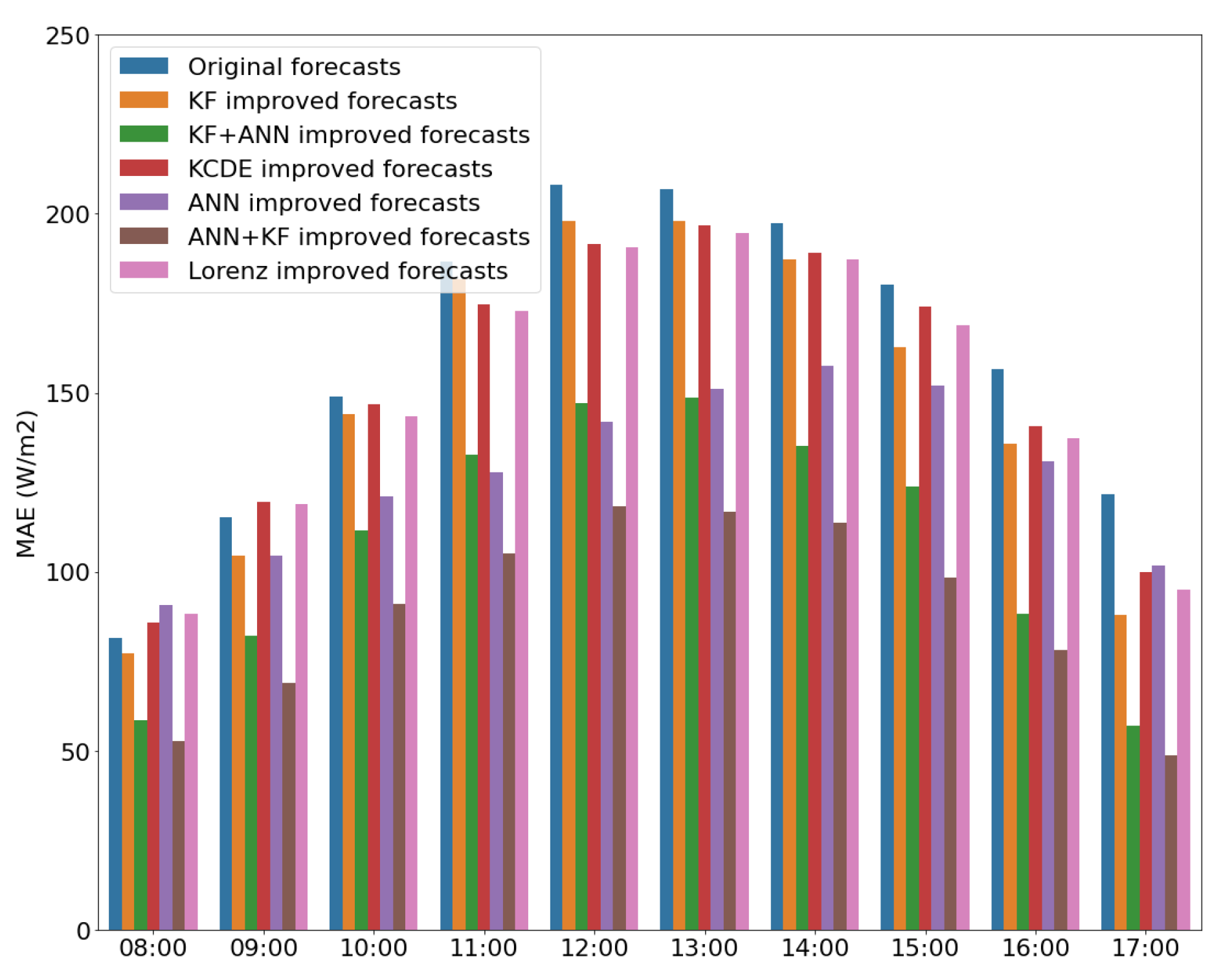
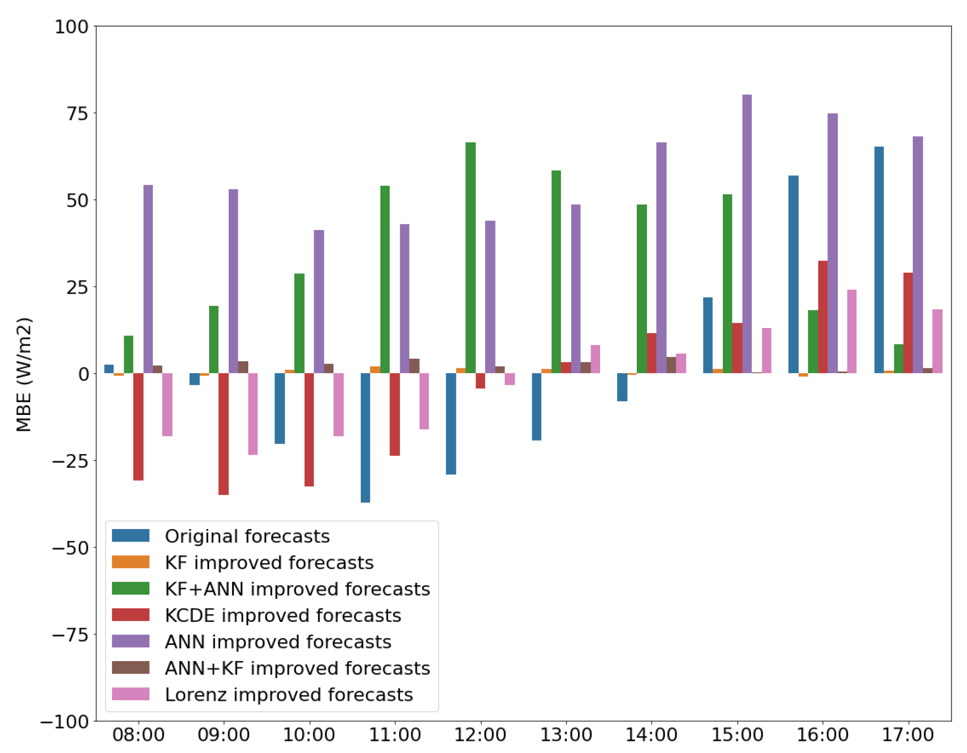
4.2. Improvements on Original Forecasts

All post-processing methods described in this study were tested on the same data and their resulting forecasts are compared by calculating the mean absolute error (MAE) and root mean squared error (RMSE) to assess the random error, and the mean bias error (MBE) to assess the systematic bias:

$$MAE=\left(\frac{1}{n}\right)\sum _{t=1}^n\left|y_t-x_t\right|$$

(10)

$$RMSE=\sqrt{\left(\frac{1}{n}\right)\sum _{t=1}^n{(y_t-x_t)}^2}$$

(11)

$$MBE=\left(\frac{1}{n}\right)\sum _{t=1}^n{y}_t-x_t$$

(12)

where, $y_t$ denotes the improved prediction and $x_t$ denotes the observation at a time step t.

The MAE of original and resulting forecasts after the application of each method is shown in Figure 4 and Figure 5 for the 10-min resolution and hourly resolution data, respectively.

Naturally, as solar irradiance presents increasingly sudden variations, the MAE is higher for fine-grained WRF forecasts.

All tested methods reduce the MAE of original WRF forecasts, the ANN presents the best reduction of the mean error for both time resolutions. However, Figure 6 and Figure 7 illustrate that the ANN is the only method that degrades the mean bias of original WRF forecasts in both time resolutions. The Kalman filter is the best method to reduce the mean bias for both time resolutions, with almost all the bias removed from original WRF forecasts.

The consecutive combination of these two methods was tested in an attempt to gather the performance of the Kalman filter in reducing the mean bias and the capability of the ANN to reduce the mean error.

The percentage improvement given by each method compared to the original WRF is described in

Table 2. Percentage improvement of each method compared to original forecasts in a 10-min resolution (the higher the better, negative values denote degraded results).

Method	MAE	RMSE	MBE
$MO{S}_{ANN}$	22	12	−95
$MO{S}_{Lorenz}$	7	10	48
KF	8	7	95
KCDE	6	9	27
KF + $MO{S}_{ANN}$	32	17	−31
$MO{S}_{ANN}$ + KF	45	41	91

and

Table 3. Percentage improvement of each method compared to original forecasts in hourly resolution (the higher the better, negative values denote degraded results).

Method	MAE	RMSE	MBE
$MO{S}_{ANN}$	37	36	−49
$MO{S}_{Lorenz}$	9	10	43
KF	13	11	94
KCDE	11	12	21
KF + $MO{S}_{ANN}$	54	50	−7
$MO{S}_{ANN}$ + KF	13	11	95

for a 10-min resolution and hourly resolution forecasts, respectively.

Focusing only on the combinations of ANN and KF methods, the results for both time resolutions reveal that when the ANN is applied lastly, it introduces a bias that was previously removed by the Kalman filter. However, when the Kalman filter is applied after the ANN in high-resolution data, it maintains the reduced mean error and additionally reduces the mean bias firstly introduced by the ANN in a 10-min resolution. Therefore, a consecutive ANN MOS post-processing followed by Kalman filtering yields the best overall results, improving the original MAE by 45% and the original MBE by 91%.

A different type of behavior could be verified in hourly resolution, where for the same combination of methods, the Kalman filter degrades the mean error previously improved by the ANN. In this time resolution, the best approach may depend on the application: if a reduced random error is preferred, a combination of KF + ANN can be used in this order, improving the original MAE by 54% even if the MBE is degraded by −7%, generating positive biased solar irradiance forecasts. On the other hand, if one wants to avoid consecutive biased forecasts (e.g., in PV power plants coupled with batteries, an overestimation of PV production may rapidly fill the batteries in real-time, leaving no capacity to absorb further errors during the day), in which case, the ANN + KF combination is more convenient, improving the MBE of original forecasts by 95% while improving the MAE by 13%.

5. Conclusions and Further Work

This study presents the best combination of post-processing methods to improve high-resolution solar irradiance forecasts generated by a WRF model. The annual meteorological simulation for 2020 at a specific location in French Guiana was analyzed. The evaluation focuses on the capability of each method to improve both the random error and mean bias of original solar irradiance forecasts. Furthermore, an identical analysis is proposed for a lower resolution version of the same forecasts, exhibiting differences in modeling and performance for each method according to the time resolution.

The methods compared in this study are well known to improve systematic and random errors individually, namely Model Output Statistics (MOS), Kalman filter (KF) and KCDE. The results reveal that any of the methods improve both errors simultaneously; however, a combination of a neural network MOS followed by a KF post-processing improves the MAE by 45% and MBE by 91% for high-resolution forecasts. In a coarser time resolution, the same combination of methods improves the MAE by 13% and MBE by 95%, and the combination in the reverse order improves the MAE by 54% independently, degrading the MBE by −7%. In this case, the most valuable combination may depend on the preferred error to be reduced, according to the downstream application.

For future development of the work, a much more extensive analysis can be conducted by comparing the methods on multiple high-resolution forecasts, generated for different locations with different climates.

References

1. Yang, D. On post-processing day-ahead NWP forecasts using Kalman filtering. Sol. Energy 2019, 182, 179–181. [Google Scholar] [CrossRef]
2. Lauret, P.; Diagne, M.; David, M. A Neural Network Post-processing Approach to Improving NWP Solar Radiation Forecasts. Energy Procedia 2014, 57, 1044–1052. [Google Scholar] [CrossRef]
3. Pereira, S.; Canhoto, P.; Salgado, R.; Costa, M.J. Development of an ANN based corrective algorithm of the operational ECMWF global horizontal irradiation forecasts. Sol. Energy 2019, 185, 387–405. [Google Scholar] [CrossRef]
4. Lima, F.J.L.; Pereira, E.B.; Martins, F.R. Forecast of Short-term Solar Irradiation in Brazil Using Numerical Models and Statistical Post-processing. In Proceedings of the EuroSun 2014 Conference, Aix-les-Bains, France, 16–19 September 2014; International Solar Energy Society: Freiburg, Germany, 2015; pp. 1–10. [Google Scholar] [CrossRef] [Green Version]
5. Barutcu, B.; Tanriover, S.T.; Sakarya, S.; Incecik, S.; Sayinta, F.M.; Caliskan, E.; Kahraman, A.; Aksoy, B.; Kahya, C.; Topcu, S. Improving WRF GHI Forecasts with Model Output Statistics. In Progress in Clean Energy, Volume 1; Dincer, I., Colpan, C.O., Kizilkan, O., Ezan, M.A., Eds.; Springer International Publishing: Cham, Switzerland, 2015; pp. 291–299. [Google Scholar] [CrossRef]
6. Diagne, M.; David, M.; Boland, J.; Schmutz, N.; Lauret, P. Post-processing of solar irradiance forecasts from WRF model at Reunion Island. Sol. Energy 2014, 105, 99–108. [Google Scholar] [CrossRef]
7. Pelland, S.; Galanis, G.; Kallos, G. Solar and photovoltaic forecasting through post-processing of the Global Environmental Multiscale numerical weather prediction model: Solar and photovoltaic forecasting. Prog. Photovoltaics Res. Appl. 2013, 21, 284–296. [Google Scholar] [CrossRef]
8. Rincón, A.; Jorba, O.; Baldasano, J.M.; Monache, L.D. Assessment of short-term irradiance forecasting based on post-processing tools applied on WRF meteorological simulations. In Proceedings of the State-of-the-Art Workshop, COST ES 1002: WIRE: Weather Intelligence for Renewable Energies, Paris, France, 22–23 March 2011; pp. 1–9. [Google Scholar]
9. Sweeney, C.P.; Lynch, P.; Nolan, P. Reducing errors of wind speed forecasts by an optimal combination of post-processing methods: Comparing and combining post-processing methods. Meteorol. Appl. 2013, 20, 32–40. [Google Scholar] [CrossRef] [Green Version]
10. Rincón, A.; Jorba, O.; Frutos, M.; Alvarez, L.; Barrios, F.P.; González, J.A. Bias correction of global irradiance modelled with weather and research forecasting model over Paraguay. Sol. Energy 2018, 170, 201–211. [Google Scholar] [CrossRef]
11. Louka, P.; Galanis, G.; Siebert, N.; Kariniotakis, G.; Katsafados, P.; Pytharoulis, I.; Kallos, G. Improvements in wind speed forecasts for wind power prediction purposes using Kalman filtering. J. Wind. Eng. Ind. Aerodyn. 2008, 96, 2348–2362. [Google Scholar] [CrossRef] [Green Version]
12. Lorenz, E.; Hurka, J.; Heinemann, D.; Beyer, H.G. Irradiance Forecasting for the Power Prediction of Grid-Connected Photovoltaic Systems. IEEE J. Sel. Top. Appl. Earth Obs. Remote Sens. 2009, 2, 2–10. [Google Scholar] [CrossRef]
13. Welch, G.; Bishop, G. An Introduction to the Kalman Filter. Proc. Siggraph Course 2006, 8, 16. [Google Scholar]
Figure 1. An example of kernel density estimation (black) generated with the help of Gaussian kernels (red) used to define the local distribution of each sample (green).
Engproc 18 00027 g001
Figure 2. Kalman filter applied operationally for the post-processing of daily-issued predictions.
Engproc 18 00027 g002
Figure 3. Solar irradiance measured in 10-min resolution (blue) and in-hourly resolution (red) during 20 January 2020.
Engproc 18 00027 g003
Figure 4. Resulting MAE per hour of the day following the application of each method and convenient combinations of methods on 10-min resolution WRF forecasts.
Engproc 18 00027 g004
Figure 5. Resulting MAE per hour of the day following the application of each method and convenient combinations of methods on hourly resolution WRF forecasts.
Engproc 18 00027 g005
Figure 6. Resulting MBE following the application of each method and convenient combinations of methods over 10-min resolution WRF forecasts.
Engproc 18 00027 g006
Figure 7. Resulting MBE following the application of each method and convenient combinations of methods over hourly resolution WRF forecasts.
Engproc 18 00027 g007