K-Means Clustering Assisted Spectrum Utilization Prediction with Deep Learning Models ^†

Abstract

The radio spectrum is a finite and scarce resource needed to transport data generated by existing and emerging wireless mobile networks and services. As the demand for wireless services is increasing, operators look for ways to efficiently utilize their assigned spectrum. While operators do regularly perform spectrum occupancy measurement using an external spectrum analyzer or installing a dedicated sensing network to understand and plan the spectrum utilization level, both in time and spatial dimensions, such a measurement-based approach is expensive, given the dynamic and wide area covered by spectrum utilization. This paper proposes an indirect approach to assess and predict the average spectrum utilization level using data traffic measured from base stations of an operator network. K-Means clustering and deep learning algorithms, namely Convolution Neural Network (CNN) and Long Short Term Memory (LSTM), are used to model and analyze the current and future spectrum utilization in the 900 MHz frequency range. Data collected from 639 base stations of a mobile operator are used to build the spectrum utilization model. The results show that the CNN model trained on clustered data outperforms the model developed on non-clustered data (with a Root Mean Square Error (RMSE) of 0.58), mainly for base station level prediction. In terms of utilization level, the results also show that the operator does not optimally utilize the 900 MHz range.

1. Introduction

Over the last three decades, cellular data traffic has exploded due to the proliferation of attractive telecom services with requirements ranging from high throughput to guaranteed low latency and low error rate. To respond to the demand, mobile network operators (MNOs) continuously upgrade their networks, e.g., by deploying advanced network technologies such as Advanced Fourth Generation Long Term Evolution (LTE+) and Fifth Generation (5G) broadband cellular mobile networks. These networks are designed to efficiently utilize the available spectrum and operate in the previously unutilized spectrum in the GHz range.

As the radio spectrum is one of the key and finite resources to transport the growing traffic, there is an ever-increasing demand for it. Due to its favorable propagation condition in providing high coverage and capacity, some bands (mostly sub-6 GHz) are being intensively utilized at different times of the day and space (e.g., location and service area), creating some sort of “scarcity”, in contrast with other bands [1]. In most cases, the non-uniformity of users’ spatial distribution and usage patterns within various geographical areas and times limits the full utilization of the available radio spectrum assigned for MNOs [2]. In order to increase the efficient use of spectrum bands, MNOs consider different spectrum harvesting approaches, such as intra or inter-operator spectrum sharing or spectrum refarming that rely on detailed knowledge about the spectrum usage in time and space.

From the MNO’s perspective, optimizing the spectrum usage focuses not only on maintaining the quality of service but also on ensuring that the allocated spectral resources can support the demands of subscribers. Thus, operators are expected to understand the dynamics of their spectral resource utilization by continuously monitoring the use in terms of space, time, and the number of channels (in a channelized band) that all users in a certain territory may access. While conducting continuous spectrum measurement by dedicating sensing networks is the most accurate approach to attaining such knowledge, it is costly and resource intensive, given cellular traffic’s rising demand and dynamic nature. Rather, an alternative approach is to exploit the correlation between spectrum use and transported data/voice traffic information, which is already available in the operator’s network, to understand, estimate, and predict the spectrum utilization.

From these aspects, several literature analyzed efficient spectrum/channel use in spectral and temporal dimensions. Motivated by the lack of knowledge regarding spectrum occupancy in South Africa, the authors of [3] measured the spectrum occupancy for Global System for Mobile Communications (GSM) 900 and 1800 MHz bands. The results indicate a maximum occupancy of 20% for UHF bands and different maximum utilization during peak hours for the GSM 900 (92%) and 1800 (40%) MHz. Similarly, spectrum utilization in Malaysia’s TV and cellular bands was carried out in [3] showing the maximum utilization of 35%, 10%, and 26% in GSM900, GSM1800, and 3G bands, respectively, and 11% and 13% utilization for TV broadcasting in VHF and UHF bands.

The practical prowess of time series modeling methodologies are considered for predicting spectrum occupancy in different bands and applications. In this regard, ref. [4] applied Autoregressive Integrated Moving Average (ARIMA) models, Lagrangian Support Vector Machine, and an Elman network (simplified models of Recurrent Neural Networks (RNNs)) are used to predict spectrum occupancy in a TV and cellular bands. The results show that the RNN technique outperforms the other models in prediction accuracy for cellular networks, as it better captures the non-stationarity and several irregularities in the data traffic. In contrast, the ARIMA model works efficiently in the TV band, since the traffic pattern is stationary. A similar analysis is presented in [5] for GSM channel utilization modeling and prediction with Seasonal ARIMA (SARIMA).

On the other hand, traffic volume and resource utilization mapping is presented in [1,6]. Traffic-related measurements such as call success rate, call drop rate, and antenna properties, including antenna height, transmit power, used/unused time, and frequency bandwidth, are used in [6] to indirectly map system/network parameters into spectrum utilization efficiency. Under a multi-MNOs environment, the analysis results showed a heavy under-utilization of the spectrum. In [1], upper limits on the traffic volume and the spectrum resource usage is evaluated for a single LTE cell to ensure seamless video streaming in dense urban environments.

While these papers indicated: (1) the need for analyzing spectrum usage directly from measurement or indirectly from voice/data traffic volume; and (2) the need for prediction or classification models that are capable of understanding random spectrum usage, there is still a limitation of capturing the spatial correlation within various geographical regions.

With the limitations in mind, the main objective of this paper is to develop a machine-learning-based model that captures the spatio-temporal variation of spectrum utilization. The model helps to understand (in an average sense) how the operator utilizes the different spectrum bands allocated to it. For that, 100 days of voice traffic channel data (hourly based frequency utilization per cell in percentage) are collected from 639 base stations operating at the 900 MHz frequency range. Based on the data, the approaches followed in this work are as follows:

• Map channel utilization measurements into spectrum utilization using an industry practiced utilization formula. Erlang B is used to validate the formula and the mapping in both cases is found to be similar;
• Temporal clustering with K-mean is applied to classify the spectrum utilization of the 639 base stations. The clustering has two-fold advantages, first to understand the spectrum utilization in decision making, such as load optimization [7] and second, to improve prediction accuracy [8];
• RNN (specifically, Long Short Term Memory (LSTM)) and Convolutional Neural Network (CNN) are applied to predict future utilization on a per cluster level;

The indirect spectrum usage assessment is of low cost and requires fewer resources, as it uses the operator’s already monitored/available data. With knowledge of the average spectrum utilization, operators may follow multiple approaches, such as going for a new frequency band in the case of “full utilization”; reframing frequency, half rate configuration implementation, and spectral efficient technologies to improve the utilization in case of moderate/medium utilization; or in the case of low utilization even allowing other users to utilize its frequency in the context of cognitive radios or spectrum sharing with other operators [9]. To the best of our knowledge, no prior work has investigated spectrum utilization based on the operator’s data. Even though our analysis considers voice traffic at 900 MHz of the spectrum channel, it can easily be extended to different spectrum bands and data traffic volume inputs with appropriate traffic-spectrum utilization mapping and more complex learning architecture.

The remainder of the paper is organized as follows. The spectrum utilization concept and its traffic mapping are discussed in Section 2. We present the clustering and prediction approaches used in Section 3, followed by the results and discussion in Section 4. Finally, we conclude the work in Section 5.

2. Spectrum Utilization Analysis

2.1. Spectrum Bands in Cellular Mobile Networks

Radio spectrum is divided into frequency/spectrum bands, e.g., in mobile systems 800 MHz, 900 MHz, 1800 MHz, 2100 MHz, and 2600 MHz bands are allocated for various generations of mobile systems [9]. Each band has different propagation characteristics and bandwidth that, in turn, determine mobile network coverage and capacity [2]. Operators further divide the frequency bands into channels (also called carriers) and are used to transport traffic and control information. As an example in GSM systems operating in the 900 MHz band, the band is further divided into 124 duplex channels (or carriers) of 200 kHz bandwidth.

By systematically spacing base stations in a geographic area, each base station is configured to operate on a certain group/cluster of channels. The configured channels are reused by other base stations as many times as the resulting co-channel interference is within the service requirement [10]. In mobile systems, channels are classified as a physical channel and a logical channel. The physical channel corresponds to one timeslot on one carrier/channel, while the logical channel reflects the specific type of information carried by the physical channel, which could be either a traffic channel or a control channel. A traffic channel in GSM is abbreviated by TCH and is used for either voice or data service. For voice service, each timeslot can carry a full rate TCH of 9600 bit/s, two half-rate TCHs of each 4800 bit/s rates, or one of the control channels.

2.2. Traffic Engineering

As previously stated, the main intention of this work is to use data available in operators’ performance report systems (PRS) to estimate current and future channel utilization. When viewed per base station level where measurement is available, channel utilization level, among others, depends on the number of configured channels per base station; the specific geographic area; time of a day; users’ behaviors; service delivered; generation of the cellular network; rate, i.e., full- or half rate, supported; and multiplexing scheme used.

Cognizant of these facts, as well as taking the availability of operator’s data and operator’s understanding, the utilization study is a 2G network providing voice service. The approach is, however, generalizable to other advanced networks and it is one area in which we are working to publish the results in the future. Moreover, from the operator’s PRS, one can collect the aggregate offered traffic, measured in Erlang, for the configured channels per base station on an hourly basis and for both full-rate, $T_{v_F}$, and half-rate, $T_{v_H}$, TCH channels. For this paper, data available per base station are TCH traffic both for half and full rate, configured channels per base station, and each site’s longitude and latitude to analyze the spatial behavior of its utilization. Six hundred and thirty-nine sites (base stations) are used and one-month data with a granularity of 1 hour is collected.

Traffic engineering is then used to map the utilized channels, which in turn will be compared with the configured channels to compute the percentage utilization. Channel utilization, $C_U$, is defined as:

$$C_U=\frac{T_{v_F}}{C_c\times \left(1+\frac{T_{v_H}}{T_{v_F}}\right)}\times 100$$

(1)

The operator understudy designed its voice service assuming Erlang B service with a grade of service of 98% network availability [9]. Figure 1 shows the calculated spectrum/channel utilization, based on Equation (1), for a particular base station.

3. Methodology

As the spectrum utilization data are evaluated from the cellular traffic observed in a timely basis, it is modeled as a non-linear and non-stationarity time series. In order to capture the commonality in users’ behaviors and distribution at different times and locations, a cluster-level approach is considered when predicting the utilization. The prediction model is developed using LSTM and CNN for clustered and non-clustered data.

3.1. Utilization Clustering with K-Means

As one of the most popular unsupervised clustering algorithms due to its simplicity and linear complexity, K-Means is widely used in many application areas such as computer vision, image processing, and business analytics [9]. The goal of the algorithm is to group the unlabeled multidimensional data into K clusters by assigning each data point to one unique cluster based on the provided features. With the objective of maximizing intra-cluster similarities and minimizing the inter-cluster similarities in the spectrum usage, we used Silhouette analysis to find the optimum number of clusters.

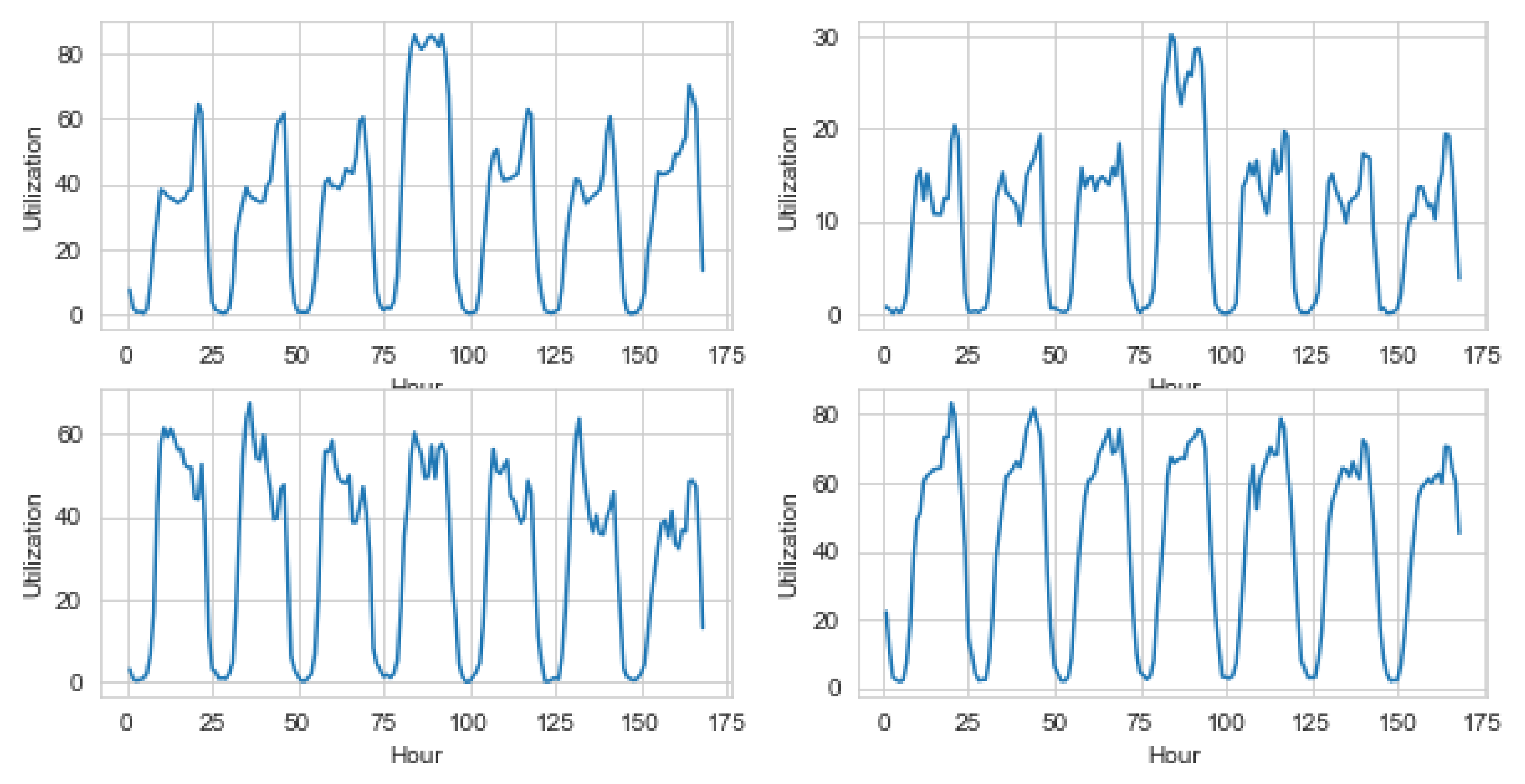
The Silhouette index (SI) is used to distinguish the different unique patterns and measures the distance between the time series and the centroid of the cluster they belong to compared through comparison with other clusters. Base stations might have significant load variation, as shown in Figure 2, due to changes in work or rest time in commercial and residential regions, as well as variations in human behavior through time and in different locations, among other factors. Based on the district pattern on the spectrum utilization time series data, SI can be used to cluster the different spatially distributed base stations. The SI for the time series dataset, y, and k the number of clusters, is defined as [9]:

$$SI\left(C\right)=\frac{1}{N}\sum _{c_k\in C}\sum _{y_i\in c_k}\frac{b(c_k,y_i)-a(c_k,y_i)}{max(a(c_k,y_i),b(c_k,y_i))}$$

(2)

where $a(c_k,y_j)=\frac{1}{|c_k|}{\sum }_{y_j\in c_k}\left|\right|y_i-y_j\left|\right|$,is the measure of similarity of the time series to its own cluster and $b(c_k,y_j)={min}_{\begin{array}{c}{c}_m\ne c_k\\ c_m\in C\end{array}}\frac{1}{|c_k|}{\sum }_{y_j\in c_k}\left|\right|y_i-y_j\left|\right|$, is the measure of dissimilarity from time series in other clusters.

3.2. Spectrum Utilization Prediction Approach with Deep Learning

The remarkable achievement of deep learning prediction in relation to wireless network problems, including its capability to capture complex nature and its processing of time series information, was achieved with a “time-aware” architecture. Without explicitly decomposing the different time series characteristics of spectrum utilization, deep learning will model/learn its dynamic temporal behavior. We consider the two widely used deep learning networks, CNN and LSTM, for the spectrum utilization problem.

3.2.1. Spectrum Utilization Modeling Using CNN

CNN is a type of deep neural network initially designed for image processing problems, but now it is applied to data that can be represented in a grid-like matrix form. In CNN, time-series and textual data can be represented by a 1D vector and a 2D matrix can be used to represent the pixels in the image data [11]. Unlike image processing, the CNN-based time series analysis/prediction requires extracting information along the time dimension, hence the reason we use the stack 1D CNN model.

To achieve the purpose of extracting features, two layers of a 1D-convolution layer are used. Max pooling layer follows each convolution layer to shirk the input resolution and assist the convolution layer to extract abundant temporal correlated features under the various input resolutions. In addition, a flattening layer for data reshaping and two dense layers are used sequentially to get the required output shape.

3.2.2. Spectrum Utilization Modeling Using LSTM

LSTM network is an advanced recurrent neural network (RNN) and is designed to learn order dependence in sequence prediction. The LSTM contains three parts, namely the Forget gate, $f_t$, Input gate, $i_t$, Output gate, $O_t$, and memory cell, $C_t$, where each part performs a separate function. The forget gate chooses whether the information coming from the previous timestamp is to be remembered or is irrelevant and can be forgotten. The input gate is used to quantify the importance of the new information carried by the input. While in the output gate, the cell passes the updated information from the current timestamp to the next timestamp. Even with its computational complexity for retaining memory, it is easy to model complex non-linear feature interactions using the LSTM [12].

$$f_t=\sigma (X_t\times U_f+H_{t-1}\times W_f)$$

(3)

$$i_t=\sigma (X_t\times U_i+H_{t-1}\times W_i)$$

(4)

$$C_t=f_t\odot C_{t-1}+i_t\odot tanh(x_t\times U_c+H_{t-1}\times W_c)$$

(5)

$$O_t=\sigma (X_t\times U_o+H_{t-1}\times W_o)$$

(6)

$$H_t=O_t\odot tanh\left(C_t\right)$$

(7)

For our real-valued prediction problem, three layers of LSTM networks are used with ReLU, $\sigma (.)=R\left(z\right)=max(0,z)$, as an activation function.

4. Results and Discussion

4.1. Experimental Settings

4.1.1. Data Preprocessing

We considered a dataset from an operator measuring the spectrum utilization of GSM 900 in Ethiopia. The data were collected for 100 days, from 1 January to 10 April 2021, with a granularity of 1 h for 639 base stations. Additionally, each site’s longitude and latitude information was taken to analyze the spatial behavior of its utilization. The operator has 61 and 85 channels configured to handle GSM service at 900 Mhz and 1800 Mhz, respectively (Tabel

Table 1. GSM channel configuration.

Network Type	Channel Type	Frequency Number
GSM 900	BCCH	14
	TCH	47
	Guard band	1
GSM 1800	BCCH	24
	TCH	61
	Guard band	1

). The maximum cell capacity for GSM900 is 8TRX per cell and 12 TRX for DCS 1800 [9].

Data preprocessing techniques, such as handling missing values, standardization, and outlier handling, are applied to the collected dataset. With that, five base stations with a continuous missing value are excluded; the data set is divided into 80% of training data, 10% of validation data, and 10% of test data.

4.1.2. Hyperparameter Tuning

Hyperparameter tuning refers to finding the best parameters to get the best results from models. Hyperparameters are set before training a machine learning model. These hyperparameters need to be optimized to adapt the model to a dataset [6].

When building the LSTM model, how many hidden layers the model will include, the number of LSTM cells that should be used in each layer, and what the dropout should be must be considered, in addition to other parameters. Similarly, the CNN model is defined with various hyperparameters such as kernel size, filter size, hidden layer, optimizer activation function, and Epoch. A grid search algorithm was used for selecting these appropriate combinations of hyperparameters listed in

Table 2. Hyperparameters used in LSTM And CNN Models.

Hyperparameters	Value
	CNN	LSTM
Hidden Layer	2	3
Number of Filters	(64), (32)	-
Kernel Size	(3), (3)	-
Hidden layer Neurons	-	(48), (32), (32)
Batch Size	64	128
Dropout	0.2%	0.2%
Maxpooling-1D	2	-
Dense layer	(50),(24)	-
Optimizer	Adam	Adam
Activation Function	ReLU	ReLU
Epoch	2000	100

as it is critical for building a model with better accuracy.

4.1.3. Evaluation Metrics

The Model evaluation aims to estimate the generalization accuracy of a model on future or test data. We jointly used two evaluation metrics to quantify our model performance: Mean Absolute Error (MAE) and Root Mean Squared Error (RMSE).

$$MAE=\frac{1}{N}\sum _{i=1}^N|y_i-{\widehat{y}}_i|$$

(8)

$$RMSE=\sqrt{\frac{1}{N}\sum _{i=1}^N{(y_i-{\widehat{y}}_i)}^2})$$

(9)

where N is the size of the evaluated set and ${\widehat{y}}_i$ is the predicted utilization for $y_i$.

4.2. Model Performances

4.2.1. Clustering with K-Means

As the utilization of the spectrum resource at a particular base station relates to the number of channels allocated and the aggregated traffic requested from the users, its temporal pattern resembles, to certain extent, the users’ behavior.

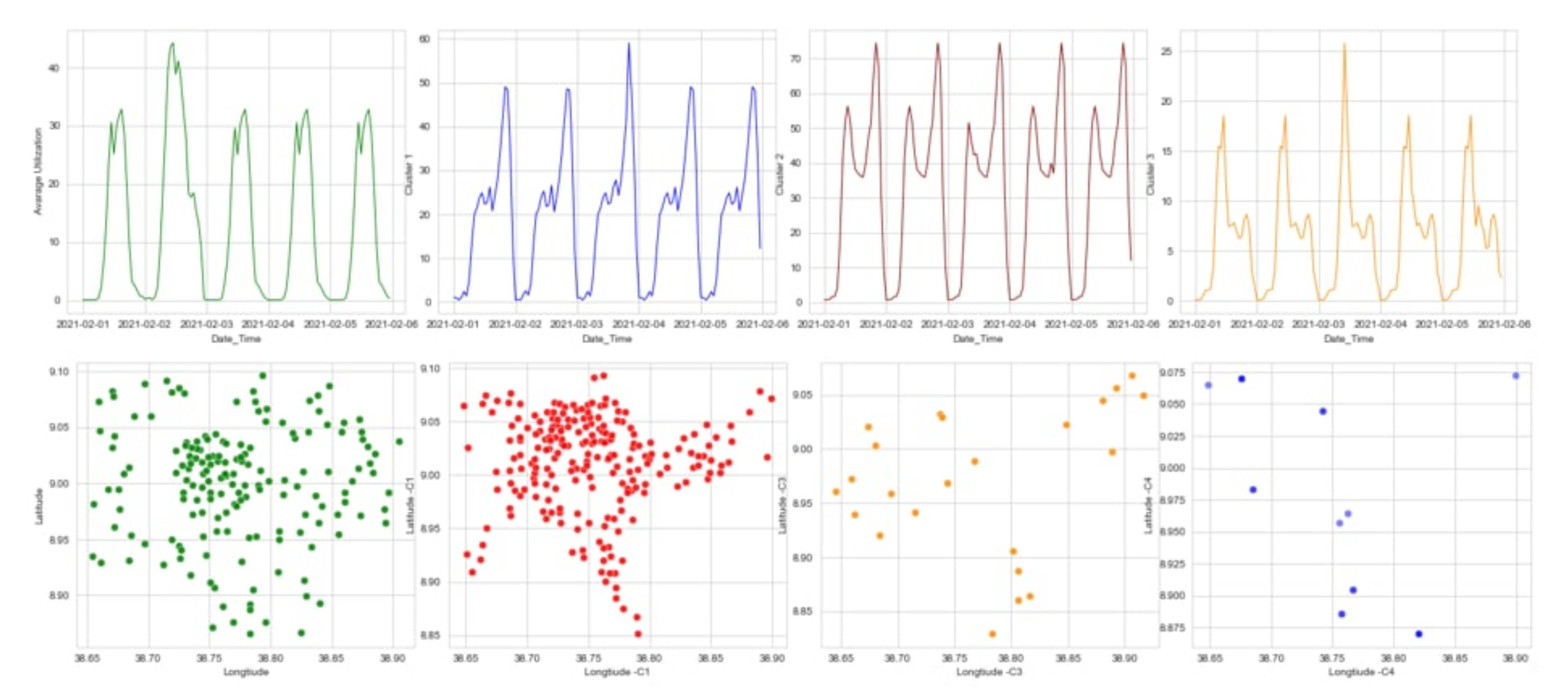
In the K-Means analysis, the closeness of the utilization pattern of a particular base station to the mean traffic pattern of a cluster is evaluated for cluster membership. Using preprocessed data, the K-Means algorithm clusters the data into an optimal cluster size of five based on the minimum SI score. Figure 3 illustrates the utilizations pattern and the spatial distribution of the corresponding base stations. The plots illustrate a distinct variation in utilization pattern due to factors such as user behavior (the high call rate during working hours indicated by the high picks) and a higher number of channel allocations (reflected in 3rd cluster, from left to right). Aside from being an input for better spectrum utilization through dynamic spectrum allocation, the clustering based approach averaged out the different patterns observed at a base station level to four, simplifying network-level predictions.

4.2.2. Prediction Performance

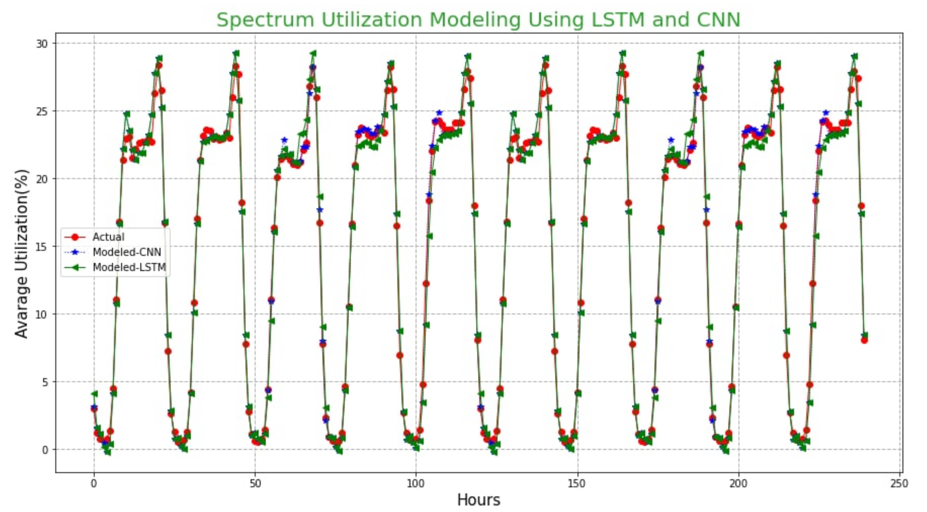
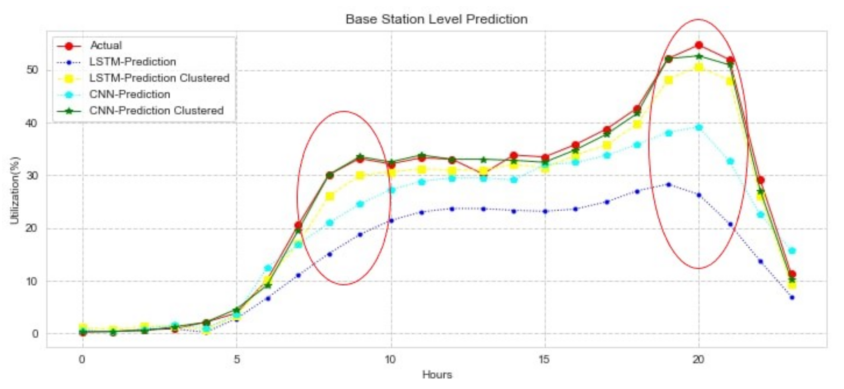
The prediction for spectrum utilization at a cluster level and base station level was made considering the two models: LSTM and CNN. Figure 4 and

Table 3. Cluster level prediction performance.

	Clustered		Non-Clustered
	RMSE	MAE	RMSE	MAE
LSTM	0.8	0.845	1.197	1.057
CNN	0.585	0.26	0.767	0.521

present results for cluster-level prediction that showed close performance between the LSTM and CNN models in capturing characteristics of the GSM 900 spectrum usage. Similarly, results for 24 h base station level prediction are shown in

Table 4. Performance evaluation results for base station level prediction.

	RMSE	MAE	MAPE	MSE
LSTM-Prediction	13.34	010.325	7.684	1.434
LSTM-Prediction Clustered	2.4492	2.092	6.872	0.641
CNN-Prediction	7.114	5.058	4.433	0.589
CNN-Prediction Clustered	1.04	0.76	2.3821	0.201

and Figure 5.

As noted, the prediction error produced by our LSTM model is much greater than the CNN (RMSE of 0.58) in both cluster and base station levels, showing its limitation was an inability to sufficiently learn the patterns (i.e., trend, seasonalities, and non-linearities) inherent in the data.

Compared to the error generated by the cluster level prediction (RMSE of 1.04), the base station level approaches in both models perform poorly. Especially during high utilization, the prediction error is very significant, which will create network condition and QoS degradation in case of prediction-based network resource allocation and optimization.

5. Conclusions

In wireless network planning and optimization, data-prediction-assisted analysis provides the opportunity for operators to determine the extent to which the resources are utilized and quality of service is attained. As spectrum is the scare resource in wireless communication, it is important for MNOs to understand how the spectrum is utilized over time and space.

In our paper, spectrum utilization data are modeled as time series data during model development, and various strategies for enhancing the model’s performance are employed to obtain a better model with the least amount of error. Since the utilization data in practice are not typically measured, we exploit the traffic utilization relation. A cluster-level approach is considered with the help of K-Means to provide network-level spectrum utilization prediction CNN and LSTM algorithms. Based on the temporal pattern, the GSM 900 band utilization is clustered into four. To compare and evaluate the prediction accuracy, four different metrics are used. As shown, the model developed for the cluster data using the CNN outperforms the LSTM algorithm with an RMSE value of 0.58. Similarly, for base-station-level prediction, CNN is found to be the best predicting model with an RMSE value of 1.04.

We hope the presented results provide a new insight for MNOs to understand the utilization level of the spectrum allocated to them that can also be extended to 3G and beyond networks. Moreover, the presented approach is on a per-cluster level, which spans a wider geographic area. How to obtain base-station-level knowledge and for a large number of base stations is another area to explore in future work.

References

1. ITU-R. Spectrum Occupancy Measurements and Evaluation; Report SM.2256-1; ITU: Geneva, Switzerland, 2016. [Google Scholar]
2. Dalela, P.K.; Nayak, A.; Tyagi, V.; Sridhara, K. Analysis of spectrum utilization for existing cellular technologies in context to cognitive radio. In Proceedings of the 2011 2nd International Conference on Computer and Communication Technology (ICCCT-2011), Allahabad, India, 15–17 September 2011; pp. 585–588. [Google Scholar]
3. Barnes, S.D.; Jansen Van Vuuren, P.A.; Maharaj, B.T. Spectrum occupancy Investigation: Measurements in South Africa. J. Int. Meas. Confed. 2013, 46, 3098–3112. [Google Scholar] [CrossRef] [Green Version]
4. Agarwal, A.; Sengar, S.; Gangopadhyay, R. Spectrum Occupancy Prediction for Realistic Traffic Scenarios: Time Series versus Learning-Based Models. J. Commun. Inf. Netw. 2018, 3, 44–51. [Google Scholar] [CrossRef]
5. Luis, P.; César, H.; Enrique, R.-C. Modeling of GSM Spectrum Based on Seasonal ARIMA model. In Proceedings of the 6th IEEE Latin-American Conference on Communications, Cartagena, Colombia, 5–7 November 2014. [Google Scholar]
6. Jordan, J. Hyperparameter Tuning for Machine Learning Models. 2017. Available online: https://www.jeremyjordan.me/hyperparameter-tuning/ (accessed on 23 January 2021).
7. Saitwal, M.S. Dynamic Spectrum Sharing between Mobile Network Operators in GSM. Ph.D. Thesis, Indian Institute of Technology Hyderabad, Telangana, India, 2015. [Google Scholar]
8. Musey, J.A.; Barlow Keener, E. The Spectrum Handbook; Summit Ridge Group, LLC: New York, NY, USA, 2018. [Google Scholar]
9. Bantigegn, F. Hybrid Clustering and Deep Learning-Based Spatio-Temporal Analysis of Spectrum Usage. Master’s Thesis, Addis Ababa University, Addis Ababa, Ethiopia, 2021. [Google Scholar]
10. Marsa-Maestre, I.; Ito, T.; Pollin, S.; Chiumento, A.; Gimenez-Guzman, J.M. Efficient spectrum usage for wireless communication. Wirel. Commun. Mob. Comput. 2019, 8719849. [Google Scholar] [CrossRef]
11. Maya, M. Convolutional neural networks for forex time series forecasting. In AIP Conference Proceedings; AIP Publishing LLC: Melville, NY, USA, 2021; Volume 2459, p. 030024. [Google Scholar]
12. Staudemeyer, R.C.; Morris, E.R. Understanding LSTM: A tutorial into Long Short-Term Memory Recurrent Neural Networks. arXiv 2019, arXiv:1909.09586. [Google Scholar]
Figure 1. Spectrum/channel utilization.
Engproc 18 00002 g001
Figure 2. Different channel utilization observed at four base stations.
Engproc 18 00002 g002
Figure 3. The four clustered base stations based on their average spectrum utilization patterns.The top-row plots representing the average utilization pattern of each cluster in five days duration, and the bottom-row plots represents the spatially distributed base stations of each cluster.
Engproc 18 00002 g003
Figure 4. Actual vs. predicted plot for CNN and LSTM.
Engproc 18 00002 g004
Figure 5. Base station level prediction with both LSTM and CNN.
Engproc 18 00002 g005