Relationship between Stationarity and Dynamic Convergence of Time Series ^†

Abstract

In economic science, when a stochastic process is studied from an econometric approach, it focuses on stationarity and the reference approach to dynamic equilibrium is ignored. Although both approaches are theoretically closely linked through the common purpose of making forecasts, in existing methodologies they are studied in a mutually exclusive way. Therefore, in this paper the consistency between dynamic equilibrium and stationarity is analyzed. In practice, the theoretical correspondence between these two important properties could present some inconsistency due to misspecification in an autoregressive model or the presence of spuriousness, generated by the components of the series.

1. Introduction

In recent years, economists have been mainly interested in the study of successions of random variables that change over time and that give rise to stochastic processes; in which, from the econometric approach, stationarity, as a particular state of equilibrium, is considered an elementary assumption in the specification of a model that has the purpose of forecasting. On the other hand, if the stochastic processes are studied from the dynamic stability approach, the fundamental assumption is convergence, which will determine the behavior of the time series through the construction of difference equations.

Although both approaches are theoretically linked, forecasting studies are carried out in different ways.

In this regard, when time series are analyzed, the estimated models aim to understand the series around its dynamic structure to make a forecast as an extrapolation of the stochastic process or time series [1,2,3,4]. The origin of the study focuses on the understanding of predictable components and time lags in dynamic analysis, which is based on the estimation of stochastic equations in differences.

From a theoretical point of view, it is accepted that there is a correspondence between dynamic convergence and stationarity, since both properties are a key point in the forecast of a realization; that is, a time series is stationary if and only if its dynamics are stable or convergent to equilibrium. For this reason, this research aims to open a line of empirical research on this correspondence.

It should be noted that in all the textbooks on the subject it is assumed that stationarity is a sufficient condition to estimate an autoregressive type model and as a result the projection of a realization is obtained.

In this regard, if the assumption of ergodicity is assumed, there is uncertainty or ambiguity in the estimation due to the high degree of complexity involved in building the probability distribution structure of a stochastic process. Consequently, when doing an empirical study, it is likely that both properties are not consistent, in an issue that has not been addressed in the conventional literature.

A solution to resolve the inconsistency may be to extract the components of the series and model only the irregular component.

2. Theoretical and Conceptual Approach on the Stationarity–Convergence Relationship

From the econometric point of view, when we talk about stationarity, the first difference of a time series is fundamental (Equation (1)), which from the dynamic stability approach represents an equation in differences. This implies that the problem of forecasting a realization in econometric terms is widely linked to the formulation and estimation of difference equations from the dynamic stability approach.

The following equation represents a stochastic process without intercept:

$$\Delta y_t=y_{t+1}-y_t$$

(1)

In this way, if the series is first order stationary, it should converge towards the dynamic stability of the process, and vice versa.

The Importance of Stationarity and Convergence in a Stochastic Process

Stationarity is a particular state of statistical equilibrium and is a fundamental part of the study of time series [5]. The probability distributions corresponding to these series remain stable over time. This is because, for any subset of the time series, the joint probability distribution must remain unchanged [6]. Furthermore, the fact that a series is stationary implies that the system is impacted by some type of shock in each instance, it will adjust to equilibrium again [7] or the consequences of impact will gradually disappear; that is, a shock in period t will have a small effect at time t + 1 and a smaller one at t + 2, and so on [8].

Since there is no variation in the probability distribution, if the time series is non-stationary, the results derived from classical linear regression are invalid or simply may not have theoretical meaning, which is known as spurious correlation [9].

To solve this problem, as defined by Granger and Newbold [10] based on the study by Yule [11], the application of cointegration models and error correction mechanism (ECM) for the long term emerged, applying the Engle and Granger [12] cointegration model for equations with two or more variables and the Johansen [13,14] model for systems of equations with autoregressive vectors. In these cases, it should be noted that, if the series are not stationary, they must be adjusted by differentiation, and with the same order to guarantee cointegration. Consequently, when we analyze the time series or stochastic process, it is of vital importance to determine stationarity by applying tests such as Phillips–Perron [15] and Augmented Dickey–Fuller [16], which are explained below.

$$Y_t=\rho Y_{t-1}+u_t$$

(2)

If $\rho =1$ it is a random walk model without intercept with the presence of a unit root; that is, the serie is not stationary; in contrast, if $\left|\rho \right|<1$ it is a stationary serie and is also convergent.

In this regard, Gujarati and Porter [17] pose an interesting question: why not simply regress $Y_t$ on its lagged value over a period $Y_{t-1}$ and find that $\rho$ is statistically equal to 1?

If this happens, $Y_t$ would not be stationary. Nevertheless, it is not convenient to estimate the regression by ordinary least squares (OLS) and test the hypothesis that $\rho =1$ through the usual t-test, since this test has a very marked bias in the case of a unit root; for this reason, Equation (2) is manipulated by subtracting $Y_{t-1}$ from both sides simultaneously to obtain Equation (3).

$$Y_t-Y_{t-1}=\rho Y_{t-1}-Y_{t-1}+u_t$$

$$\Delta Y_t=\left(\rho -1\right)Y_{t-1}+u_t$$

$$\Delta Y_t=\delta Y_{t-1}+u_t$$

(3)

Therefore, the regression is not estimated on Equation (2), but on Equation (3), and the null hypothesis $\delta =0$ is tested.

As Equation (2) is a first-order difference equation, it is required that it meets the stability condition $\left|\rho \right|<1$ as mentioned [4].

From the dynamic stability approach, the solution of a random walk model without drift seen as a difference equation is:

$$y_t=A{b}^t$$

(4)

where $A=y_0,b=a_0$.

Thus, the path described by Equation 4 depends on the value of b. In this case, if the complementary function tends to zero when t grows indefinitely, the equilibrium is dynamically stable; that is, the trajectory expressed in Equation (4) must be analyzed as t increases as shown in

Table 1. Trajectory behaviors.

b-Value	Behavior
b > 0	Non-oscillatory
b < 0	Oscillatory
|b| > 1	Divergent
|b| < 1	Convergent

[18].

In the same way, derived from Equation (4), when stipulating the convergence condition of the time trajectory $y_t$ towards the equilibrium $y_p$ we must rule out the case of $b=\pm 1$, which means that there is a unit root from the point of view econometric.

In general terms, the necessary and sufficient equilibrium condition is confirmed for a trajectory to be convergent if and only if |b| < 1, according to the stationarity condition.

3. Empirical Evidence of Bias in the Stationarity–Convergence Relationship

In order to find possible empirical inconsistencies between dynamic convergence and stationarity in a time series, three stochastic processes corresponding to trade between Mexico and China were analyzed to which the unit root test was applied and their convergence was analyzed at equilibrium using first-order autoregressive models.

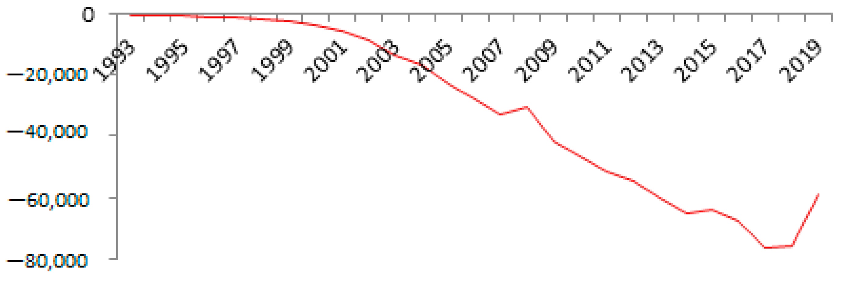
3.1. Case 1: Trade Balance of Mexico with China: An Explosive Deficit Balance

In this first case, the trade balance between Mexico and China was analyzed, explained by the difference between Mexico and China in millions of dollars per year in the period 1993–2020. Figure 1 shows that the deficit for Mexico systematically increases explosively over time, so it is evidently a non-stationary and divergent stochastic process.

Table 2. DFA test results.

Case 1	Coefficient	Confidence	t-Statistics	p_Value
Y(−1)	0.0330		1.2890	0.9459
	(1.28)	1%	−2.6534
		5%	−1.9539
		10%	−1.6096
Case 2	Coefficient	Confidence	t-Statistics	p_Value
Y(−1)	−0.0162		−0.4544	0.8856
	(−0.45)	1%	−3.6999
C	−2639.322	5%	−2.9762
	(1.878)	10%	−2.6274
Case 3	Coefficient	Confidence	t-Statistics	p_Value
Y(−1)	−0.2525		−1.8578	0.6481
	(−1.85)	1%	−4.3393
C	2325.362	5%	−3.5875
	(0.75)	10%	−3.2292
@Trend	−837.7699
	(−1.79) *

* t-statistic for statistical significance in parentheses.

shows the results obtained in the Dickey–Fuller augmented (DFA) test using the E-views software, with the t-statistic in parentheses.

The case 1 is discarded since $=\left(\rho -1\right)=0.0330$. $\rho =1.0330>1$. In the remaining cases, we can verify that, according to the hypothesis test, the null hypothesis is not rejected; consequently, the series has a unit root; additionally, despite the fact that the coefficient is negative and greater than −2, they are not statistically significant, so we can conclude that it is a divergent and non-stationary stochastic process in congruence with what is stipulated in the theory.

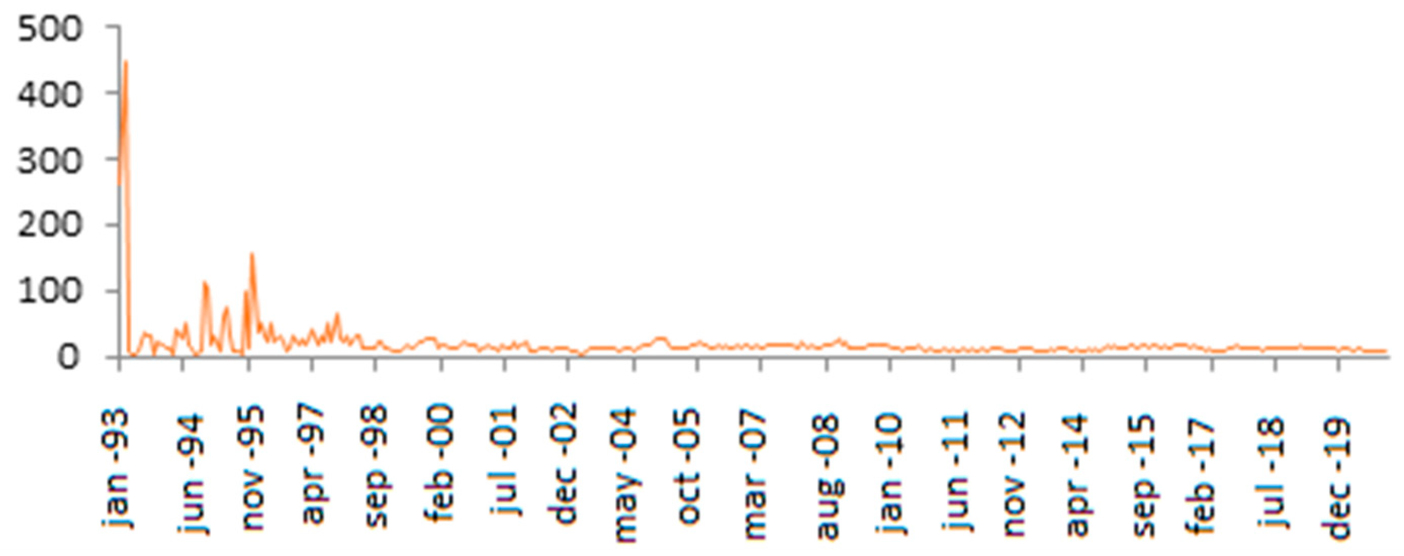
3.2. Case 2: Trade Balance of Mexico with China: An Estimate in Relative Terms

In this second case, it is proposed to use the trade balance in relative terms; that is, the quotient between imports and exports made by Mexico with its second trading partner on a monthly basis (Figure 2).

Similarly,

Table 3. DFA test results.

Case 1	Coefficient	Confidence	t-Statistics	p_Value
Y(−1)	−0.4609		−11.3628	0.0000
	(−11.36)	1%	−2.5719
		5%	−1.9418
		10%	−1.6161
Case 2	Coefficient	Confidence	t-Statistics	p_Value
Y(−1)	−0.6093		−13.6917	0.0000
	(−13.69)	1%	−3.4497
C	10.3563	5%	−2.8700
	(6.52)	10%	−2.5713
Case 3	Coefficient	Confidence	t-Statistics	p_Value
Y(−1)	−0.6500		−14.1956	0.0000
	(−14.19)	1%	−3.9857
C	18.7574	5%	−3.4233
	(6.05)	10%	−3.1346
@Trend	−0.0456
	(−3.14) *

* t-statistic for statistical significance in parentheses.

shows the results obtained in the unit root test with δ coefficients between −2 and 0, which is why not one of them is discarded. The best model that describes the trajectory is case 2, according to the criteria of Akaike, Schwartz, and Hannan-Quinn and it is obtained that $\rho =0.3907$, which shows that the convergence and stability condition is met, $\left|\rho \right|<1$ and similarly, from the econometric approach, $\delta$ is statistically significant, in addition, the p-value of the test is 0.0000, so the existence of a unit root is rejected. We can then conclude that it is a stationary and convergent stochastic process.

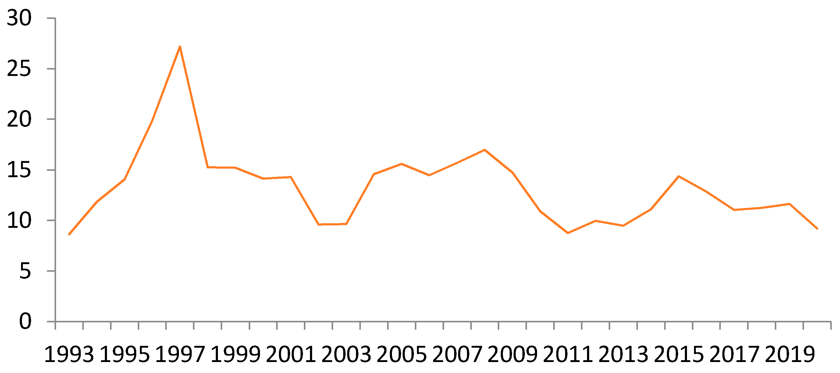
3.3. An Empirical Inconsistency in the Fluctuation of Trade between Mexico and China

In a third case, the behavior of the trade balance between Mexico and China in the period 1993–2020 was analyzed with annualized data.

In the first instance, if we inspect the graph in Figure 3, we can see that the series is possibly stationary and convergent.

Table 4. DFA test results.

Case 1	Coefficient	Confidence	t-Statistics	p_Value
Y(−1)	−0.0321		−0.6413	0.4300
	(−0.64)	1%	−2.6534
		5%	−1.9539
		10%	−1.6096
Case 2	Coefficient	Confidence	t-Statistics	p_Value
Y(−1)	−0.4470		−2.7081	0.0857
	(−2.70) *	1%	−3.6999
C	6.0326	5%	−2.9763
	(2.61) *	10%	−2.6274
Case 3	Coefficient	Confidence	t-Statistics	p_Value
Y(−1)	−0.5746		−3.4853	0.0613
	(−3.48) *	1%	−4.3393
C	10.21	5%	−3.5875
	(−3.53) *	10%	−3.2292
@Trend	−0.1756
	(−2.16) *

* t-statistic for statistical significance in parentheses.

shows that for the three cases a negative value of δ and greater than −2 was obtained.

As can be seen, the p value in all three cases is greater than 0.05; therefore, at 95% confidence, the null hypothesis that there is a unit root is not rejected, thus, the analyzed series is not stationary.

However, if we analyze in detail the dynamic equilibrium in the three cases, the value of δ is negative, greater than −2 and statistically significant for cases 2 and 3, which means that the series in question is convergent.

If we opt for case 3, according to the value of the t statistic and the p value, we can assert that the coefficient of $\delta$ is statistically significant at 95% confidence; likewise, we determine the value of $\rho$ which is 0.4254, implies that the series is convergent and stable. It is important to mention that by choosing case 3 convergence is guaranteed but around a deterministic trend, and consequently the stability of the series is questioned.

For case 2, the coefficient $\delta$ is also statistically significant from which a value of p of 0.5530 is derived; that is, the convergence and stability of the series is confirmed again. However, when applying the unit root test, it was shown that the series is non-stationary, both at 99% and 95% confidence level.

From the econometric approach, in the case of annual figures, the stability of the series would be ambiguous since it is not a stationary series since it is not possible to reject the null hypothesis of the unit root test.

4. Concluding Remarks

When theoretically analyzing the stochastic processes, the results obtained were consistent for the divergent case; however, for the convergent case certain ambiguities were found.

We can then assert that there is a double causal relationship between stationarity and dynamic stability theoretically. Because the forecasts about the behavior of the series are the result of making estimates using a stationary series, in autoregressive models, this statement is of great importance. However, the problem arises when there is no stationarity.

Then, we can conclude that the non-stationarity of a series could mean a wrong specification of the model, including a spurious correlation. So, when applying the model for projections of series or forecasts, in the bias with respect to the true values, the impact is not necessarily lost over time. In other words, the possible dynamical convergence that follows from a non-stationary series might not be the closest to the true trajectory; in short, it could be classified as a false dynamic convergence.

Let us also consider that within the process to determine stationarity, if we assume the assumption of ergodicity, stationarity implies a simplification of various assumptions; in general, that a sample preserves the properties of the population.

In other words, the ergodicity assumption implies that the series is stationary, which induces a considerable homogeneity in the stochastic process, reduces the uncertainty as a simplification of the suppositions. So, if the analyzed series is not stationary, the ergodicity is not satisfied; therefore, the assumptions are not simplified and, consequently, there would be no stability and convergence in the series, so the coefficients obtained from the regression are the result of spuriousness or an erroneous specification of the model.

Finally, since the simplification of the assumptions is not met, the mean and variance of the series vary with respect to time; then, being non-stationary, the ergodic process is not fulfilled, and they should not be used for forecasts.