Abstract
The presence of non-stationarity can have crucial effects on statistical tests on correlation between two or more data sets. We present a procedure to detect changes in the strength of dependence between data sets that is based solely on a comparison of the ordinal structures within a moving window and thus compares the up-and-down behavior only. Hence, it is not distracted by changes within a single data set, such as change-points and trends or even nonlinear transformations, leading to non-stationarity. The applicability of the method is demonstrated for a hydrological data set of runoff time series which are impacted by a reservoir. It is demonstrated that the method overcomes problems of classical methods when non-stationarity is present.
1. Introduction
In various applications, the co-movement of different data sets is a desirable property. More often, it is a source of risk:
- If a trader holds a portfolio of various assets which are strongly ‘correlated’, it is more likely that several of them fall into the abyss at the same time.
- If a company produces parts for cars (for different brands), this company will be in trouble if the whole car industry goes through rough times.
- If several catchments in a basin are affected by extreme floods or extreme low flows at the same time, severe damage can be expected for the downstream catchments by flood superposition or spatial drought.
- If many requests are made to the same server at the same time, it becomes overloaded.
In all of these cases, it is important to monitor the strength of the interdependence between the data sets. This interdependence or co-movement is often modeled using the mathematical concept of correlation. However, sometimes it is not clear whether the time series admit second moments. Hence, it might be the case that correlation between the random variables (of which the time series consist) is not even defined. Another drawback of this mathematical concept is that it is well known to measure mostly linear dependence whilst the dependence in our applications could be far from being linear.
Our aim in the present article is to detect changes within the dependence structure between data sets. Since co-monotonic behavior might be a source of risk, we would like to detect whether this becomes (at a certain point in time) stronger or weaker. An additional difficulty arises since some of the data examples we have in mind are known to be non-stationary. Usually, tests for change points in the dependence structure require that the single time series are stationary (cf. e.g., [1,2]). If this was not the case, the tests would falsely detect a change in the dependence, which in fact might be a change in one of the single time series while the dependence between the time series remains constantly strong.
Due to climate change, the demand of being able to detect changes in the dependence structure in non-stationary settings has increased. Several data sets (like temperature) which were known to be stationary (up to some seasonal components) have started to increase systematically. Sometimes, it is not known how strong the incline of the new deterministic component is. Even worse: the incline itself is subject to change and increases stronger and stronger.
In the following, we will always use the term ‘time series’ if we consider the mathematical model, that is, a stochastic process defined on a probability space . In contrast to this, we write ‘data set’ for the real or simulated data we are using. Here, and in what follows, we always consider two time series or two data sets at a time. If we want to analyze the dependence of more than two time series or data sets, we consider them pairwise.
Let us start with a simulated example illustrating the above idea. Consider two correlated ARMA(1,1) time series, i.e.,
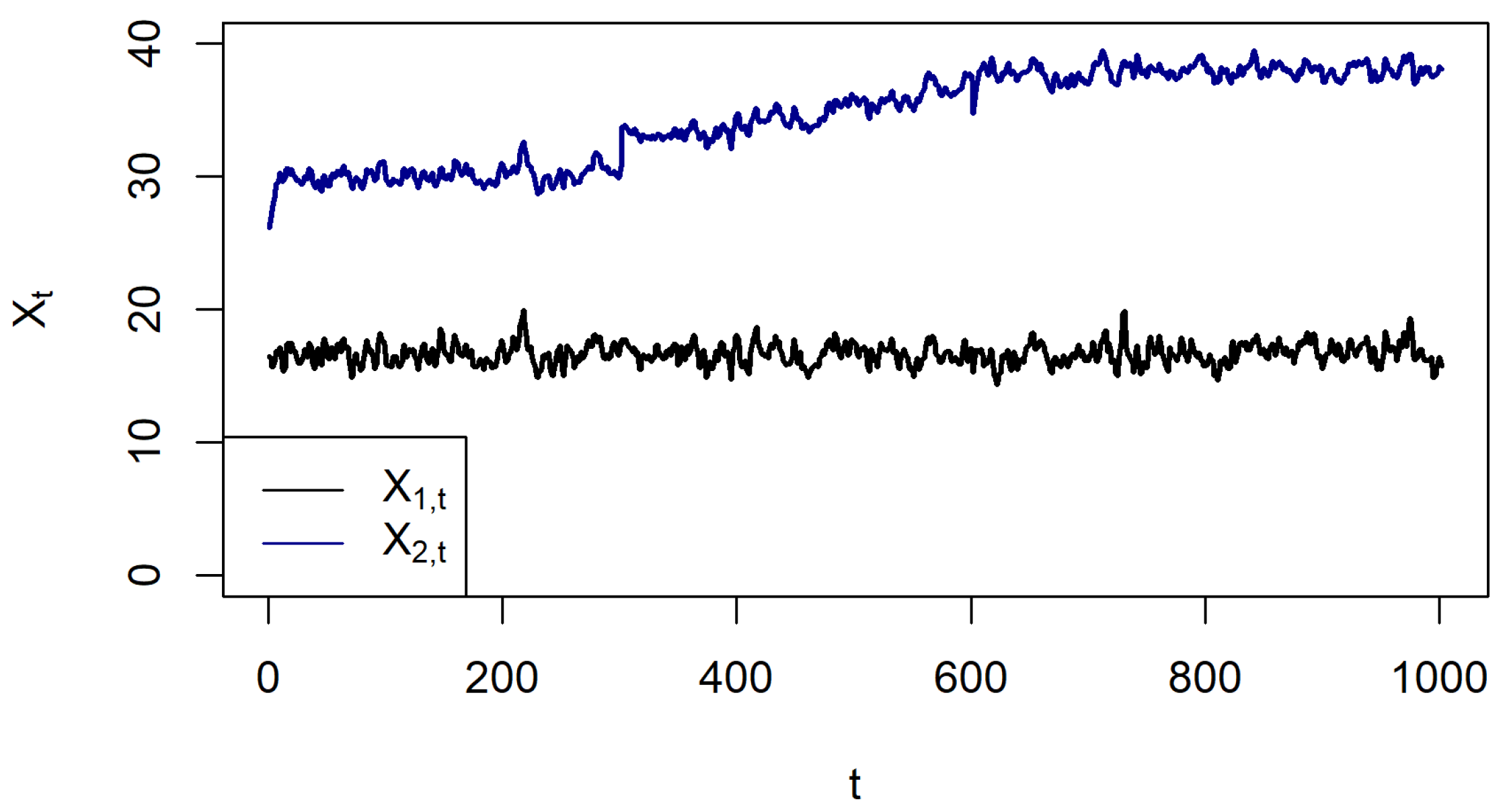
where , and with . Here, we chose , , , , , , and to simulate data points from a short-range dependent time series with a high cross-correlation (Figure 1). Artificially, two change-points were included in the data set: first, an exponential drift was added to the second part of , i.e., for and for . Secondly, another 400 data points were added (third part) by simulating once again two cross-correlated ARMA(1,1) time series and with the same parameters as before but . These two data sets were added to the first two data sets such that each set consists of 1000 data points, e.g., for and for . Moreover, the mean of the second time series was adjusted to match the exponential drift, that is, for . The exponential drift in the second series led to significant non-stationarity (detected with Mann–Kendall test for short-range dependent data; [3]). In a way, this is more than just a random simulated example: think about a data set of monthly temperature and the corresponding discharges of a river. While it is known that temperature tends to increase for most parts of the world, this was not detected yet for discharge [4], though both data sets are clearly cross-correlated. Application of the classical correlation measures such as Pearson’s correlation coefficient, , or Spearman’s Rho, denoted by , leads to a significant drop of the estimated correlation coefficients when applying the measure to the first and second part of the data. For the first part of the time series, both correlation measures detected significant correlation, where and . However, when considering also the part with the exponential drift, significant correlation was no longer detected: and . This implies that, though the correlation between both time series is still high, in the sense that they show the same up-and-down behavior, the drift masks this correlation for the classical correlation measures.
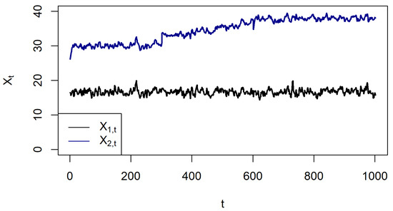
Figure 1.
Simulated cross-correlated ARMA(1,1) series with exponential drift in the middle part of the second time series.
We would like to overcome this problem. To this end, we use so-called ordinal patterns in order to analyze the up-and-down behavior of the data sets (and time series) under consideration.
The most common approach in ordinal pattern analysis works as follows: One decides for a small number , that is, for the length of the data windows under consideration. In each window, only the ordinal information is considered. There are various ways to encode the ordinal information of a d-dimensional vector in a pattern. Here, we use the following: Let denote the set of permutations of , which we write as d-tuples containing each of the numbers exactly one time. By the ordinal pattern of order d of the vector , we refer to the permutation
which satisfies
When using this definition, it is often assumed that the probability of coincident values within the vector is zero. Allowing for coincident values would require an additional convention like if for or an approach as in [5].
Roughly speaking, ordinal pattern dependence measures how often we encounter the same patterns at the same time considering our two data sets (cf. Figure 2); the theoretical counterpart is the probability
for the underlying models, that is, the time series we consider.
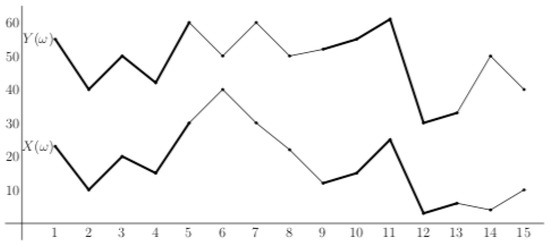
Figure 2.
Two data sets with partially co-monotonic behavior.
In fact, one subtracts the probability for the hypothetical case of independence and divides by some normalizing factor in order to obtain values between zero and one in the case of positive dependence. The mathematical definition of ordinal pattern dependence can be found in the subsequent section.
In our simulated toy example above, the ordinal pattern dependence (we have chosen ) is not impacted by the exponential drift. In fact, the ordinal pattern dependence (here, we use the sample version defined below Equation (2)) does not change significantly with and . However, the change of dependency between both time series in the last part is clearly detected with . This change can also be detected by the classical correlation measures and , but less clearly with and . Recall that, although the up-and-down-behavior remains the same in the second part, the classical measures do not detect this any more due to the moderate exponential drift in the background.
The origin of the concept of ordinal patterns lies in the theory of dynamical systems [6,7]. They have been used in order to analyze the entropy of data sets [8] and to estimate the Hurst-parameter of long-range dependent time series [9,10]. Furthermore, related methods have proved to be useful in the context of EEG-data in medicine [11], index data in finance [12] and flood data in extreme value theory [13]. Already in [14], we have suggested using ordinal patterns for the analysis of hydrological time series. Changes in the dependence have not been considered in that article. However, changes in a single data set have been analyzed in [15] via ordinal patterns. Analyzing changes in the dependence between time series/data sets is a topic that has attained considerable interest over the last few years (cf. [1,2,16]). There exists an approach (cf. [17]) that was developed to detect changes in the dependence structure despite having non-stationarity of the single time series using the concept of local stationarity, but the assumptions are rather technical and make it hard to apply to short time series in practice.
Using ordinal patterns in order to analyze the dependence between time series, instead, has several advantages: we do not need to assume the existence of second moments and the time series do not necessarily have to be stationary. Furthermore, the method is robust against small noise and/or measurement errors and the intuitive concept makes it easy to apply in practice. Since only the order structure is considered, the algorithms are quick.
The notation we are using is more or less standard. denotes a probability space in the background. We write for the expected value w.r.t. , while denotes the positive integers starting with one.
2. Methodology
Let and be two time series defined on a common probability space . We describe our analysis step-by-step:
- (I)
- Preparation and first analysis.
Check whether the whole time series are stationary. Maybe even the bivariate time-series is stationary. In this case, both single time series are stationary and the dependence structure remains the same over time. In this case, we are done. If the single time series are stationary, but the bivariate one is not stationary, one can use our method or one of those found in the literature (cf. [1,2,16]) to detect changes in the dependency. The most interesting case for us is if the two time series X and Y or at least one of them is not stationary. Then, the classical methods cannot be applied. Still, one might be interested in the analysis of co-monotonic behavior and in changes of this behavior.
- (II)
- Calculate the ordinal pattern dependence of the whole time series.
At first, we have to check whether the two time series admit ordinal pattern dependence.
Definition 1.
We define the ordinal pattern dependence between two random vectors and by
This definition of ordinal pattern dependence only considers positive dependence, which is in line with our considerations in the present article. Negative dependence could be included by analyzing the co-movement of and or by using an analogous definition taking inverse patterns into account. Usually, one is interested in measuring either positive or negative dependence. If one wants to consider both dependencies at the same time, the quantity
where for every , is useful (cf. [18]).
For data sets, we use the estimators
for and ()
for . For OPD in Equation (1), we use these plug-in estimators and denote it with .
- (III)
- (Check whether the dependence changes over time.
Using a test statistic of the following kind, we analyze whether the ordinal pattern dependence between the time series remains more or less the same
which is a CUSUM type test statistic. In the examples of the subsequent section, we already have a good candidate for the time of the structural break. If this was not the case, the argmax could be used in order to find this point in time.
3. Results
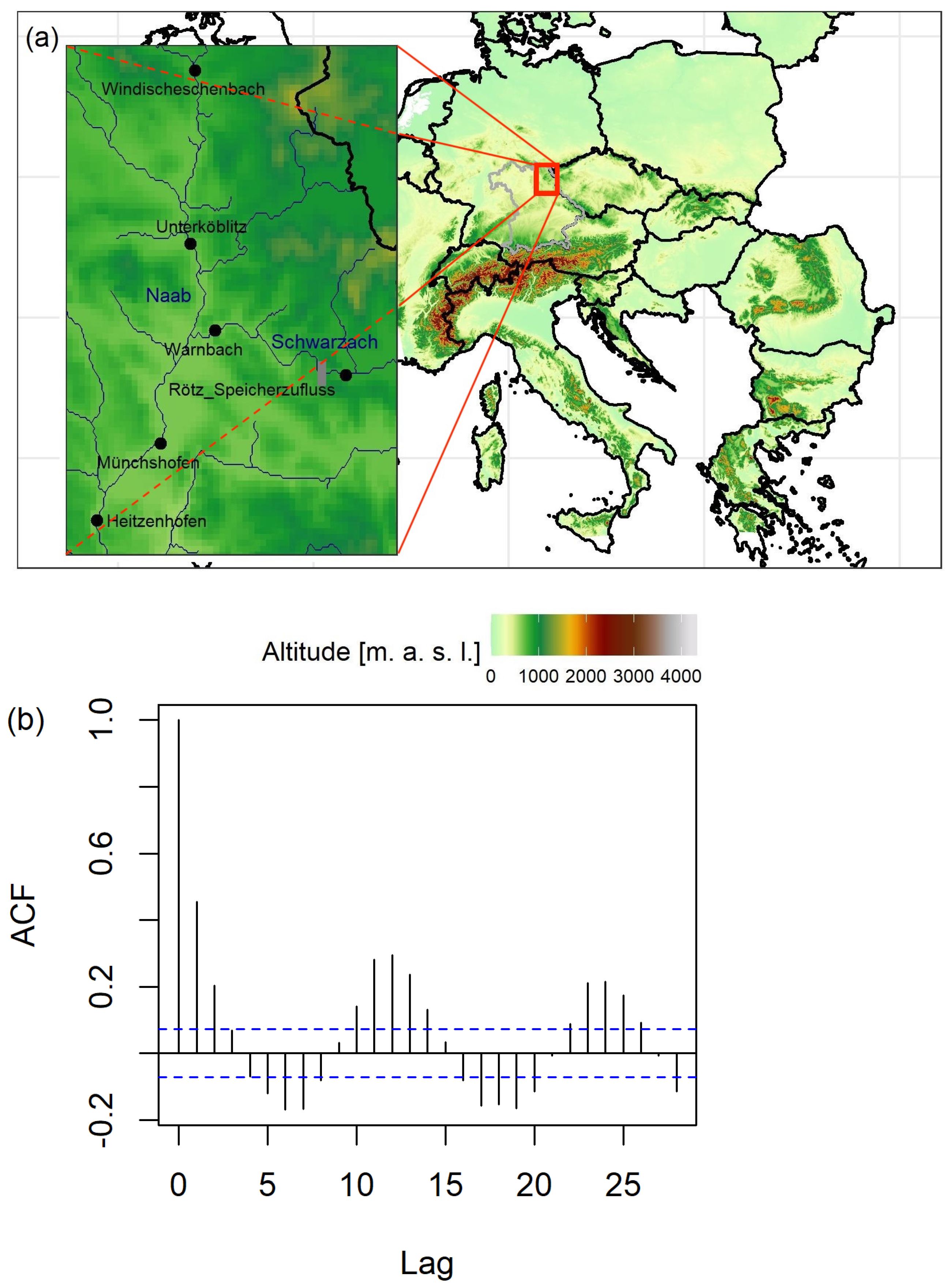
As a real life example, we consider the six runoff data sets of catchments of the mesoscale in Bavaria, Southern Germany. Four of the measuring gauges, Windischeschenbach, Unterköblitz, Münchshofen, and Heitzenhofen, are located at the main river Naab, a large tributary of the Danube river (Figure 3a). Between Unterköblitz and Münchshofen gauges, the tributary river Schwarzach flows into the Naab. Two gauges are located at the Schwarzach river: Rötz and Warnbach. In November 1975, a large reservoir was built at the Schwarzach river, called the Eixendorfer See, located directly downstream of the Rötz gauge. It serves flood protection, low water elevation (water regulation), hydropower generation, and recreation, and, with a storage of 19.30 million , it is among the largest reservoirs in Southern Germany. We consider the monthly maximum discharges of the period from 1959–2018, which often serve as a basis for flood frequency analyses. Due to their temporal resolution, monthly maximum discharges are usually considered to be short-range dependent [19] and affected by seasonality (Figure 3b).
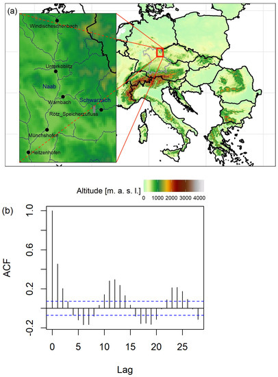
Figure 3.
(a) Map of the location of the gauges considered in the application with Bavarian borders (grey) and location of the zoom-in map in Europe (red); (b) auto-correlation of the monthly maximum discharges at Münchshofen gauge.
We apply the methods to analyze the data sets as described in Section 2.
- (I)
- Preparation and first analysis.
The available discharge data sets are checked for consistency and trimmed to a joint time period between 1959 and 2018, therefore consisting of data points each. For each data series, the Wilcoxon test for short-range dependent data [20] is applied to test whether there is a significant change-point in the mean. For the gauges Münchshofen and Heitzenhofen in the Naab river as well as Warnbach in the Schwarzach river, such a significant change-point ( significant level) was detected in the period of 1975 till 1977. This change-point can be directly related to the beginning of operation of the dam in the Schwarzach, which has a large impact on the mean since the largest discharge peaks are reduced by the reservoir for flood protection. Therefore, all gauges located downstream of the reservoir can be considered as non-stationary. Hence, the classical tests for structural breaks in the dependence structure cannot be applied.
- (II)
- Calculate the ordinal pattern dependence of the whole time series.
In the next step, we calculate the ordinal pattern dependence between the discharge series of all six gauges as given in Definition 1 with . A similar pattern length was chosen before in the case of hydrological data and proved to be sufficient (cf. [5,14]). One could also think about using and thus taking into account the annual cycle. However, this would increase the number of patterns and thus the computational effort significantly. Moreover, the annual cycle is not equally strong everywhere, e.g., due to different periods of snowmelt, and thus a general definition could be difficult. We can assume a positive dependence in this application since discharges will most likely increase and fall similarly due to spatial extension of weather patterns such as rainfall.
The ordinal pattern dependence between all six gauges is given in Table 1.

Table 1.
Ordinal pattern dependence of all six gauges for the time period 1959-2018. Since the OPD is symmetric, only the upper half of the table is shown.
The results reveal that there is a high dependence between the gauges of the main river, decreasing with distance. This can be related to weather patterns such as rainfall events which are spatially extended and affect several catchments at the same time as well as routing. Interestingly, the gauges of the tributary are less correlated, neither with each other nor with the main river. However, dependency increases for the gauges downstream of the tributary, which is hydrologically reasonable.
- (III)
- Check whether the dependence changes over time.
The commissioning of the dam in 1975 may not only affect the mean of the discharge series. Indeed, it is also likely that the dependence structure between the discharge series of the gauges is altered by it. It can be assumed that especially the dependency between the gauges upstream of the dam and therefore those not affected by the regulation have a higher dependency to the gauges downstream after commissioning of the dam since the incoming tributary discharge is regulated and smoother and thus does not alter the main river discharge as much as before. The dam may also affect the low dependency between the gauges in the tributary given in Table 1. This hypothesis is tested in the following by applying the ordinal pattern dependence to the time series before as well as after the assumed change-point in 1975 (Table 2). Due to the nature of ordinal patterns, this change-point detection is not affected by the previously detected change in mean.
Table 2.
Ordinal pattern dependence of all six gauges for the time period 1959–1975 (upper table) and 1976–2018 (lower table).
There are clear differences between the dependency before and after the commissioning of the dam. It is not straight-forward to determine if the differences are significant, since classical tests like Fisher’s Z-test cannot be applied. However, it was shown in previous studies that such differences appear to be significant ([14]). Indeed, the dependency between the upstream main river gauges, Windischeschenbach and Unterköblitz, increases or stays the same compared to the period before the commissioning of the dam. The dependency between the gauge upstream of the dam, Rötz, and downstream of the dam, Warnbach, instead decreases since the discharge is no longer transferred directly between the gauges, but the dam now regulates the runoff. Instead, the discharge of the downstream gauge is mostly impacted by inter flow. We also tested possible change-points in 1976 and 1977, taking into account a possible delayed reaction, but the general tendency of all results stayed the same. The ordinal pattern dependence, therefore, was able to detect the changes in the dependence structure caused by the commissioning of the dam despite the change in mean at the exact same position in the time series.
4. Discussion
Our method shows how the commissioning of the dam has changed the dependence between the discharge data sets. In a similar way, it could be used on the other frameworks described in the Introduction. If we had not known in advance when the dam was built, we could have analyzed this by calculating the argmax of the test statistic (3) above.
The data analysis shows that ordinal pattern dependence can indeed be used in order to derive changes in the dependence structure between time series. The method is robust, easy to implement and has the advantage that the concept behind it has a simple intuitive meaning: if the ordinal patterns are often the same at the same time points, the up-and-down-behavior of the two data sets is similar.
We have chosen here . This value has proven to be useful in the context of discharge data. Smaller values of d are more often used in statistical frameworks, while higher values are used in the analysis of dynamical systems. Finding an optimal choice for d is part of ongoing research.
In a way, our toy example and the real world data analysis of Section 3 serve as a pilot study, showing the applicability of the method. By now, it is not possible to derive critical values or confidence bands. This is not in the scope of the present paper, since it is very technical and still a work in progress: in order to leave classical stationarity behind, a standing assumption would be ‘ordinal pattern stationarity’. One needs to show that both data sets might be realizations of ordinal pattern stationary time series. Then, and that is a point being missing in the existing literature, one needs to derive limit theorems for, say, a short range dependent time-series on the space of ordinal patterns (which is a discrete space without canonical order). Finally, one might be able to derive exact change point tests in this framework. If the original time series can be assumed to be stationary, limit results like in [18] could be applied. However, the above example shows how nicely the method can deal with non-stationary time series.
Author Contributions
Conceptualization, A.S. and S.F.; methodology, A.S.; software, S.F.; writing—original draft preparation, A.S. and S.F.; writing—review and editing, A.S. and S.F.; visualization, A.S. and S.F. All authors have read and agreed to the published version of the manuscript.
Funding
This research was funded by the German Reserach Foundation (DFG) Grant No. FOR 2416 (research unit SPATE) for Svenja Fischer and Grant No. SCHN 1231-3/2 for Alexander Schnurr.
Institutional Review Board Statement
Not applicable.
Informed Consent Statement
Not applicable.
Data Availability Statement
Publicly available datasets were analyzed in this study. These data can be found here: https://www.nid.bayern.de/abfluss (accessed on 12 May 2022).
Acknowledgments
We are grateful to Bayerisches Landesamt für Umwelt, www.lfu.bayern.de (accessed on 12 May 2022), for providing the discharge data. We would like to thank three anonymous referees for their valuable comments.
Conflicts of Interest
The authors declare no conflict of interest.
References
- Aue, A.; Hörmann, S.; Horvath, L.; Reimherr, M. Break detection in the covariance structure of multivariate time series models. Ann. Stat. 2009, 37, 4046–4087. [Google Scholar] [CrossRef] [Green Version]
- Dehling, H.; Vogel, D.; Wendler, M.; Wied, D. Testing for changes in Kendall’s tau. Econom. Theory 2017, 33, 1352–1386. [Google Scholar] [CrossRef] [Green Version]
- Hamed, K.H.; Rao, A.R. A modified Mann–Kendall trend test for autocorrelated data. J. Hydrol. 1998, 204, 182–196. [Google Scholar] [CrossRef]
- Sharma, A.; Wasko, C.; Lettenmaier, D.P. If Precipitation Extremes Are Increasing, Why Aren’t Floods? Water Resour. Res. 2018, 54, 8545–8551. [Google Scholar] [CrossRef]
- Schnurr, A.; Fischer, S. Generalized ordinal patterns allowing for ties and their applications in hydrology. Comput. Stat. Data Anal. 2022, 171, 107472. [Google Scholar] [CrossRef]
- Bandt, C. Ordinal time series analysis. Ecol. Model. 2005, 182, 229–238. [Google Scholar] [CrossRef]
- Bandt, C.; Shiha, F. Order Patterns in Time Series. J. Time Ser. Anal. 2007, 28, 646–665. [Google Scholar] [CrossRef]
- Bandt, C.; Pompe, B. Permutation entropy: A natural complexity measure for time series. Phys. Rev. Lett. 2002, 88, 174102. [Google Scholar] [CrossRef] [PubMed]
- Sinn, M.; Keller, K. Estimation of ordinal pattern probabilities in Gaussian processes with stationary increments. Comp. Stat. Data Anal. 2011, 55, 1781–1790. [Google Scholar] [CrossRef]
- Betken, A.; Buchsteiner, J.; Dehling, H.; Münker, I.; Schnurr, A.; Woerner, J. Ordinal Patterns in Long-Range Dependent Time Series. Scand. J. Stat. 2020, 48, 969–1000. [Google Scholar] [CrossRef]
- Keller, K.; Unakafov, A.; Unakafova, V. Ordinal Patterns, Entropy, and EEG. Entropy 2014, 16, 6212–6239. [Google Scholar] [CrossRef]
- Schnurr, A. An Ordinal Pattern Approach to Detect and to Model Leverage Effects and Dependence Structures between Financial Time Series. Stat. Pap. 2014, 55, 919–931. [Google Scholar] [CrossRef] [Green Version]
- Oesting, M.; Schnurr, A. Ordinal Patterns in Clusters of Extremes of Regularly Varying Time Series. Extremes 2020, 23, 521–545. [Google Scholar] [CrossRef]
- Fischer, S.; Schumann, A.; Schnurr, A. Ordinal Pattern Dependence Between Hydrological Time Series. J. Hydrol. 2017, 548, 536–551. [Google Scholar] [CrossRef] [Green Version]
- Unakafov, A.; Keller, K. Change-point detection using the conditional entropy of ordinal patterns. Entropy 2018, 20, 709. [Google Scholar] [CrossRef] [PubMed] [Green Version]
- Wied, D.; Dehling, H.; van Kampen, M.; Vogel, D. A fluctuation test for constant Spearman’s rho with nuisance-free limit distribution. Comput. Stat. Data Anal. 2014, 76, 723–736. [Google Scholar] [CrossRef] [Green Version]
- Dette, H.; Wu, W.; Zhou, Z. Change point analysis of correlation in non-stationary time series. Stat. Sin. 2019, 29, 611–643. [Google Scholar] [CrossRef] [Green Version]
- Schnurr, A.; Dehling, H. Testing for Structural Breaks via Ordinal Pattern Dependence. JASA 2017, 112, 706–720. [Google Scholar] [CrossRef] [Green Version]
- Wu, C.L.; Chau, K.W.; Li, Y.S. Predicting monthly streamflow using data-driven models coupled with data-preprocessing techniques. Water Resour. Res. 2009, 45. [Google Scholar] [CrossRef] [Green Version]
- Dehling, H.; Fried, R.; Wendler, M. A robust method for shift detection in time series. Biometrika 2020, 107, 647–660. [Google Scholar] [CrossRef]

Publisher’s Note: MDPI stays neutral with regard to jurisdictional claims in published maps and institutional affiliations. |
© 2022 by the authors. Licensee MDPI, Basel, Switzerland. This article is an open access article distributed under the terms and conditions of the Creative Commons Attribution (CC BY) license (https://creativecommons.org/licenses/by/4.0/).