Proceeding Paper

Blind Image Separation Using the JADE Method †

1
Department of Electronics, Faculty of Technology, Mohamed Boudiaf University, M’Sila 28000, Algeria
2
LIS Laboratory, Department of Electronics, Faculty of Technology, Ferhat Abbas University, Setif 19000, Algeria
*
Author to whom correspondence should be addressed.
Presented at the 1st International Conference on Computational Engineering and Intelligent Systems, Online, 10–12 December 2021.
Eng. Proc. 2022, 14(1), 20; https://doi.org/10.3390/engproc2022014020
Published: 28 February 2022

Abstract

:
Blind source separation (BSS) concerns the signal processing techniques that aim to find several elementary components of sources from linear combinations of these sources received on several sensors. This paper presents a method for the extraction of these independent components. It is called Joint Approximate Diagonalization of Eigenmatrices (JADE) and uses fourth-order cumulants. A simulation example shows the performance of the proposed algorithm by displaying its high separation accuracy. The proposed technique is compared to the Equivariant Adaptive Source Separation Algorithm (EASI).

1. Introduction

In signal and image processing, there are many cases where a set of observations are available and from which we wish to recover the sources that generated them. This problem, which has become a hotspot in the field of signal processing, is known as blind source separation (BSS). It has received great attention in several research fields such as speech, sound, image, telecommunications and biomedicine [1,2,3,4]. New research has significantly improved both the BSS theory and its practical applications. In biomedicine, the applications of BSS range from medical engineering to neuroscience. In image processing, BSS is a method of recovering the original images from the observed mixed images. This is referred to as blind image separation. One way to achieve the separation is to utilize relative motions of layers. Several technologies have been proposed to extract motions from image sequences [5,6]. They focus only on motion, whereas the layer restoration is not considered. Independent component analysis (ICA) has often been regarded as an attractive solution to the blind image separation problem. In biomedical applications, ICA has been applied to functional magnetic resonance imaging (fMRI) data analysis. In addition, some proposed image separation applications have taken a Bayesian approach [7]. In [4], Kayabol et al. approved a Markov random field (MRF) model to preserve the spatial dependence of neighboring pixels (e.g., sharpness of edges) in a 2-D model. They provided a full Bayesian solution to image separation using Gibbs sampling. Another MRF-based method has been proposed by Tonazzini et al. in [8]. In mechanical systems, BSS is used to evaluate complex mode shapes which may occur in the real world [9]. Also, evolutionary algorithms such as the Genetic algorithms (GA) [10,11,12,13], the Particle Swarm Optimization (PSO) algorithm [14,15,16], the Artificial Bee Colony (ABC) algorithm [17] and the JADE algorithm [18] are useful to solve optimization problems in diverse fields. They have been applied to find the optimal separation matrix in BSS techniques.
In this paper, the JADE algorithm [18] is used to solve the problem of blind source separation.
The rest of this paper is organized as follows: Section 2 describes the BSS model and the JADE algorithm. In Section 3 we present the simulation results. The conclusion and future work are given in the last section.

2. BSS Model

In a source separation situation, the observed data are composed of { X i } i = 1 , , m , where { X i } is a row-vector. The linear instantaneous mixed model of BSS can be indicated as:
X i ( t ) = j = 1 n a j i s j ( t ) ,
where a j i ( i = 1 , , m ,   j = 1 , , n ) are mixing parameters, s ( t ) = [ s 1 ( t ) , , s n ( t ) ] T are source signals, i.e., the observed signals. Then the Equation (1) can be written as:
X ( t ) = A . s ( t )
where A is the mixing matrix A m × n , and s ( t ) m × n is the source vector. In this paper, we suppose that the number of sources, n, is equal to the number of mixtures, m. Our objective is to separate the signals from each other. The order of the estimated signals is not necessary. There are many different algorithms to accomplish blind source separation. The general concept to determine independent components is to compute the separating matrix W i . The component signals are retrieved from the mixed signal by:
y = W i . X
The basic model of blind source separation is given in Figure 1.

2.1. Joint Approximate Diagonalization of Eigenmatrices

An important contribution in blind source separation is the JADE algorithm [18] which optimizes a contrast function using a fourth-order cumulant. Our objective is to develop the approach relating to JADE. The algorithm is in several stages.

2.1.1. Whitening of X

The objective of whitening is transforming the observed vector X linearly so that we get a new vector X ˜ which is white, i.e., its components are uncorrelated, and their variances are equal to unity. In other words, the covariance matrix of X ˜ is equal to the identity matrix:
E ( X . X ˜ ) = I

2.1.2. Cumulant Calculations

In the previous step, X has been transformed into a set of principal components afflicted with equal variance, P w . The objective of the JADE algorithm is to find the rotation of P w , therefore its column vectors are independent. In this algorithm, for every observed signal, the cumulants of the signals are calculated, and are placed in a fourth-order tensor. If the signals are independent, their fourth-order cumulant will be zero.
The fourth-order cumulant of a vector X can be defined as:
c u m 4 { x , x , x , x } = E { x 4 } E 2 {   x 2 }

2.1.3. Decompose the Cumulants

In the JADE method, the fourth-order cumulant is first decomposed into a set of n ( n + 1 ) 2 orthogonal eigenmatrices, n . n . This is done by forming a set of n ( n + 1 ) 2 . symmetrical orthogonal matrices and projecting the cumulant tensors onto these planes. Every element of the cumulant j is then projected onto each M i matrix:
for i = 1 to n ( n + 1 ) 2 , matrix = M i ;
for i 1 = 1 to n , and for i 2 = 1 to n
M i ( i 1 , i 2 ) = s u m ( s u m ( k ( i 1 , i 2 , : , : ) × m a t r i x )
where cumulant.

2.1.4. Joint Diagonalization of the Eigenmatrices

The diagonalization of eigenmatrices is established on the Jacobi algorithm in order to minimize the sum of squares of the off-diagonal elements that correspond to the fourth-order cumulants between the different signals. Orthogonal diagonal eigenmatrices M i are then acquired.
In Figure 2 we show the graphical representation of the JADE algorithm. The rotation matrix produces independent vectors by the diagonalization of the matrices derived from the fourth-order cumulant. A projection of the matrix of whitened scores U w onto this space will therefore produce the separating matrix, W .

2.2. Algorithm

In this section, a blind source separation method using JADE is proposed.
  • Normalize the N images.
  • Mixed images are formed by linearly mixing with a random matrix.
  • Initialization, estimate a Whitening matrix w ˜ , z = w ˜ . X .
  • Estimate a maximal set M i of cumulants matrix.
  • Find the rotation matrix V ˇ such that the simulants matrix are as diagonal as possible
    V ˇ = a r g m i n i o f f ( V + M i V )
  • Estimate A as, A = V ˇ . W 1 , and estimate the components as y = A 1 X .

3. Simulation

With the purpose of explaining the proposed technique, two images, “Lena” and “Lynda”, N = 259 × 194 , are mixed with
A = [ 0.6 0.4 0.4   0.6 ]
The performance of separated images is evaluated by using peak signal to noise ratio (PNSR) [19], which is defined as follows, and shown in Table 1, Table 2, Table 3 and Table 4.
P N S R = 10 log [ 255 m = 1 M n = 1 N s ( m , n ) y ( m , n ) ]
Experience 1: Parrot.jpg and fruit.jpg.
Experience 2: barbara.jpg, lena.jpg.

4. Discussion

From the simulation results, we can deduce:
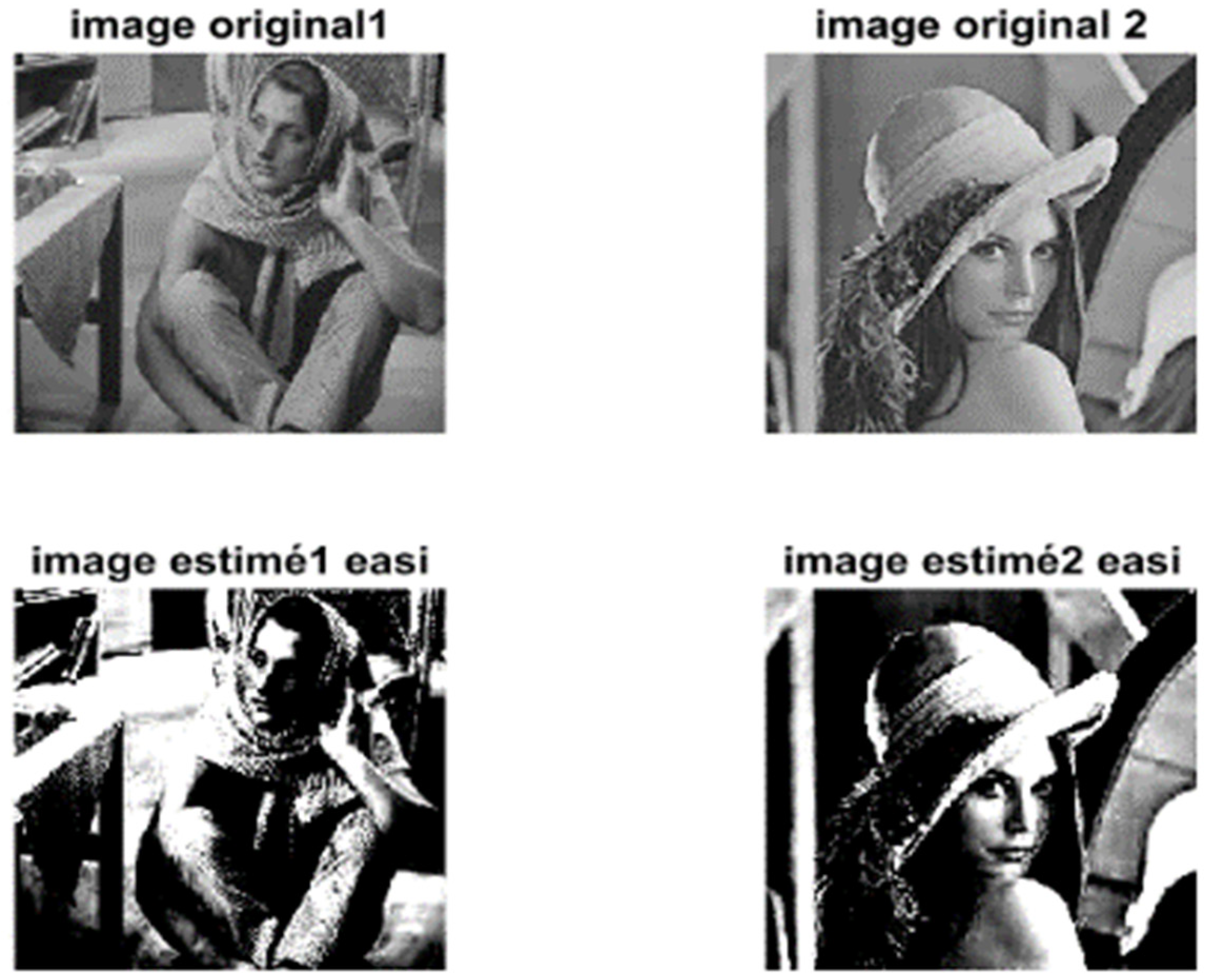
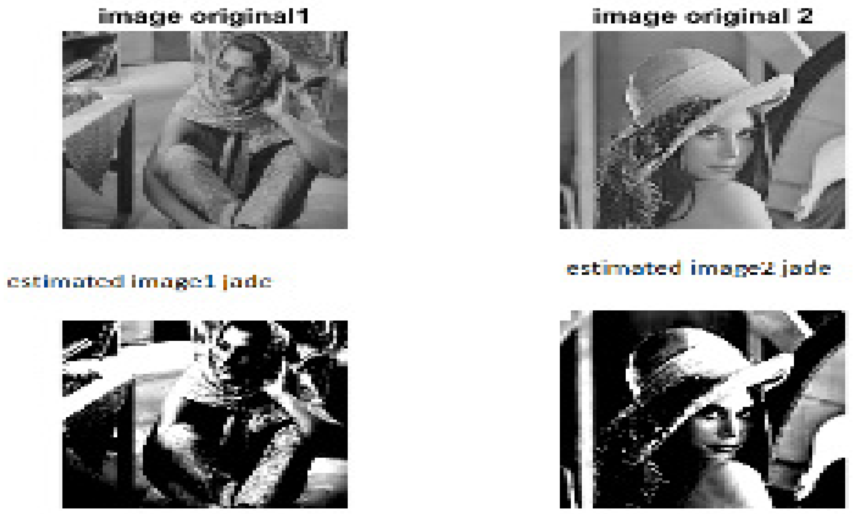
In Figure 3, Figure 4, Figure 5 and Figure 6, we see that the images of the recovered images signal resemble the original ones. Second, we demonstrate the efficacy of the proposed algorithm by using the performance index PNSR.

5. Conclusions

In this is paper, we have presented a powerful technique for natural mixtures accompanied by a blind separation of images. This technique utilizes the JADE algorithm that has low computational complexity. To evaluate the performance of the implemented JADE algorithm, a mixture of two images was used. In our future work, we will investigate other methods, such as optimization algorithms, in order to improve their performance accuracies.

Author Contributions

Conceptualization, K.A. and A.N.; methodology, K.A. and A.N.; software, K.A. and K.E.; validation, K.A., A.N. and K.E.; formal analysis, K.A.; investigation, K.A. and K.E.; resources, K.A.; data K.A.; writing—original draft preparation K.A. and A.N.; writing—review and editing, K.A., A.N. and K.E.; visualization, K.A.; supervision, K.A.; project administration, K.A.; funding acquisition, K.A., A.N. and K.E. All authors have read and agreed to the published version of the manuscript.

Funding

This research received no external funding.

Institutional Review Board Statement

Not applicable.

Informed Consent Statement

Not applicable.

Data Availability Statement

Not applicable.

Conflicts of Interest

The author declares no conflict of interest.

References

  1. Hesse, C.W.; James, C.J. On semi-blind source separation using spatial constraints with applications in EEG analysis. IEEE Trans. Biomed. Eng. 2006, 53, 2525–2534. [Google Scholar] [CrossRef] [PubMed]
  2. Kayabol, K.; Kuruoglu, E.E.; Sankur, B. Bayesian separation of images modeled with MRFs using MCMC. IEEE Trans. Image Process 2009, 18, 982–994. [Google Scholar] [CrossRef] [PubMed] [Green Version]
  3. Lin, Q.H.; Yin, F.L.; Zheng, Y.R. Secure image communication using blind source separation. In Proceedings of the IEEE 6th Circuits and Systems Symposium on Emerging Technologies: Frontiers of Mobile (IEEE Cat. No. 04EX710), Shanghai, China, 31 May–2 June 2004; pp. 261–264. [Google Scholar]
  4. Murata, N.; Ikeda, S. An on-line algorithm for blind source separation on speech signals. In Proceedings of the Nolta98, Crans-Montana, Switzerland, 14–17 September 1998; pp. 923–926. [Google Scholar]
  5. Jung, T.P.; Makeig, S.; Humphries, C.; Lee, T.W.; Mckeown, M.J.; Iragui, V.; Sejnowski, T.J. Removing electroencephalographic artifacts by blind source separation. Psychophysiology 2000, 37, 163–178. [Google Scholar] [CrossRef] [PubMed]
  6. Milles, J.; Van Der Geest, R.J.; Jerosch-Herold, M.; Reiber, J.H.; Lelieveldt, B.P. Fully automated motion correction in first-pass myocardial perfusion MR image sequences. IEEE Trans. Med. Imaging 2008, 27, 1611–1621. [Google Scholar] [CrossRef] [PubMed]
  7. Ichir, M.M.; Mohammad-Djafari, A. Hidden Markov models for wavelet-based blind source separation. IEEE Trans. Image Process. 2006, 15, 1887–1899. [Google Scholar] [CrossRef] [PubMed] [Green Version]
  8. Tonazzini, A.; Bedini, L.; Salerno, E. A Markov model for blind image separation by a mean-field EM algorithm. IEEE Trans. Image Process. 2006, 15, 473–482. [Google Scholar] [CrossRef] [PubMed]
  9. Huang, W.; Wu, S.; Kong, F.; Wu, Q. Research on Blind Source Separation for Machine Vibrations. Wirel. Sens. Netw. 2009, 1, 453–457. [Google Scholar] [CrossRef] [Green Version]
  10. Yang, Y.; Wang, X.; Zhang, D. Blind Source Separation Research, based on the Feature Distance Using Evolutionary Algorithms. Int. J. Acoust. Vib. 2014, 19, 276. [Google Scholar] [CrossRef]
  11. Malhotra, R.; Singh, N.; Singh, Y. Genetic Algorithms: Concepts, Design for Optimization of Process Controllers. Comput. Inf. Sci. 2011, 4, 39. [Google Scholar] [CrossRef]
  12. Burke, E.K.; Burke, E.K.; Kendall, G.; Kendall, G. Search Methodologies, Introductory Tutorials in Optimization and Decision Support Techniques; Springer: Berlin, Germany, 2005; pp. 97–125. [Google Scholar]
  13. Zheng, P.; Liu, Y.; Tian, L.; Cao, Y. A Blind Source Separation Method Based on Diagonalization of correlation Matrices and Genetic Algorithm. In Proceedings of the Fifth World Congress on Intelligent Control and Automation, Hangzhou, China, 15–19 June 2004; Volume 3, pp. 2127–2131. [Google Scholar]
  14. Zhou, H.; Chen, C.Z.; Sun, X.M.; Liu, H. Research on Blind Source Separation Algorithm Based on Particle Swarm Optimization. Adv. Mater. Res. 2014, 989–994, 1566–1569. [Google Scholar] [CrossRef]
  15. Bai, Q. Analysis of particle swarm optimization algorithm. Comput. Inf. Sci. 2010, 3, 180. [Google Scholar] [CrossRef] [Green Version]
  16. Tripathi, P.K.; Bandyopadhyay, S.; Pal, S.K. Multi-Objective Particle Swarm optimization with time variant inertia and acceleration coefficients. Inf. Sci. 2007, 177, 5033–5049. [Google Scholar] [CrossRef] [Green Version]
  17. Ebrahimzadeh, A.; Mavaddati, S. A novel technique for blind source separation using bees colony algorithm. Elsevier Swarm Evol. Comput. 2014, 14, 15–20. [Google Scholar] [CrossRef]
  18. Rutledge, D.N.; Bouveresse, D.J. Independent components analysis with jade algorithm. Trac Trends Anal. Chem. 2013, 50, 22–32. [Google Scholar] [CrossRef]
  19. Jyothirmayi, M.; Kuzhali, E.S.; Selvi, S. Blind Source Separation Using Forward Difference Method (FDM). Signal Image Process. 2011, 2, 121. [Google Scholar]
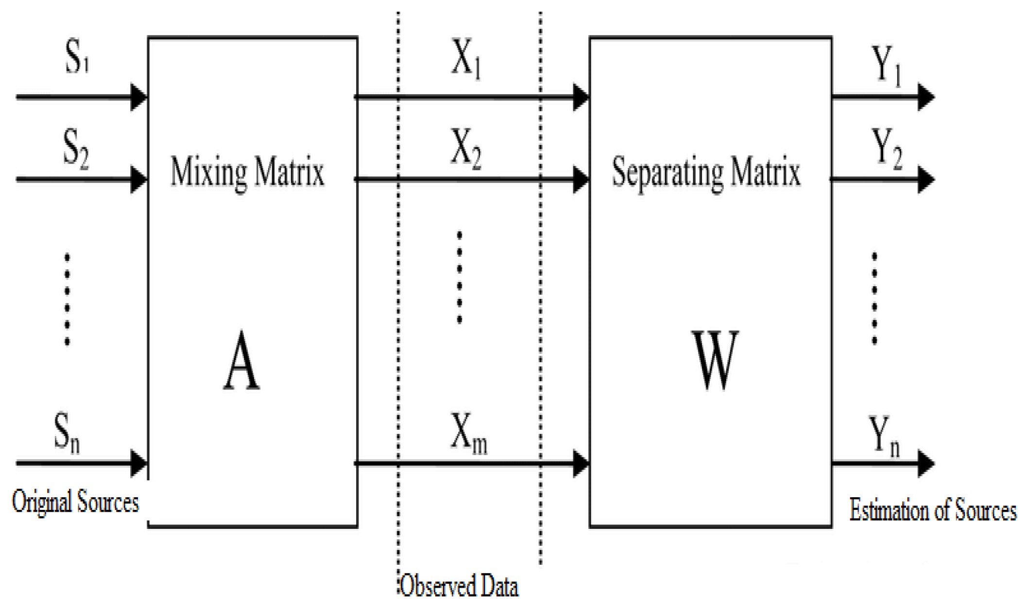
Figure 1. The basic model of blind source separation.
Engproc 14 00020 g001
Figure 2. Graphical representation of the JADE algorithm [18].
Engproc 14 00020 g002
Figure 3. EASI method.
Engproc 14 00020 g003
Figure 4. JADE method.
Engproc 14 00020 g004
Figure 5. EASI method.
Engproc 14 00020 g005
Figure 6. JADE method.
Engproc 14 00020 g006
Table 1. PNSR (dB) for the EASI algorithm.
estimated image1 EASI6.4374
estimated image2 EASI24.3083
Table 2. PNSR (dB) for JADE the algorithm.
estimated image1 JADE17.3639
estimated image1 JADE52.2668
Table 3. PNSR (dB) for the EASI algorithm.
estimated image1 EASI18.5680
estimated image2 EASI30.1416
Table 4. PNSR (dB) for the JADE algorithm.
estimated image1 JADE31.0534
estimated image2 JADE29.7526
Publisher’s Note: MDPI stays neutral with regard to jurisdictional claims in published maps and institutional affiliations.