Numerical Analysis of Heat Transfer in Nanofluids Flowing over a Stretching Surface Under the Influence of Oscillating Magnetic Fields: Application of the Crank–Nicolson Finite Difference Method ^†

Abstract

Nanofluids, which are suspensions of nanoparticles within base fluids, are employed in industries such as electronics, automotives, nuclear power, and defense to enhance thermal management, mass transfer, and microchip cooling. This study investigates heat transfer generation on a stretching sheet incorporating aluminum oxide ${(\mathrm{A}\mathrm{l}}_2{\mathrm{O}}_3)$ and magnetite ${(\mathrm{F}\mathrm{e}}_3{\mathrm{O}}_4)$ nanoparticles under conditions of constant and varying wall temperatures. Key factors considered include variable viscosity, a periodic magnetic field, and thermal radiative flux, underscoring the thermal advantages of nanoparticles in nuclear reactor applications. The Crank–Nicolson method, an implicit finite difference technique, was utilized to solve the mathematical model, with partial differential equations discretized and approximated using an explicit method. An explicit iterative method was employed to solve the momentum and energy equations in a Python solver, while boundary values were analytically resolved based on discretized equations. In the explicit method, values at the subsequent time step (n + 1) were directly computed from the current time step (n) values. This approach necessitated a sufficiently small time step to satisfy the Courant–Friedrichs–Lewy (CFL) condition for numerical stability. The study examined the mass and heat transfer characteristics of a magnetizable nanofluid. While nanoparticles enhanced heat transfer, magnetic interactions, viscosity, and thermal radiation impeded it. A periodic magnetic field was applied perpendicularly to the plates with a constant pressure gradient, utilizing a magnetic phase angle to decelerate and control flow and heat convection modulation.

1. Introduction

Preserving energy is sometimes more crucial than generating it, since energy loss is directly associated with an increase in entropy. Thus, minimizing entropy generation is crucial for achieving optimal performance in thermodynamic and heat transfer systems [1]. The employment of nanoparticles in heat transfer, particularly in water-cooled nuclear reactors, has attracted significant attention due to the enhanced thermal conductivity and improved cooling efficiency of nanofluids [2,3,4]. Nanofluids exhibit distinct properties compared to conventional solid–liquid mixtures. The enhancements result from the increased surface area of nanoparticles and the enhanced interaction between fluid molecules and solid particles at the nanoscale, which together boost heat transfer [5,6]. Nanofluids are seen as a promising approach for improving thermal management in high-heat-flux systems, such as nuclear reactors [3,4]. Despite their advantages, the stability of nanofluids remains a considerable challenge; processes including aggregation and sedimentation may diminish their heat conductivity and durability [2].

The behavior of nanomaterials under irradiation in nuclear environments is a significant subject. Recent study indicates that exposure to intense neutron irradiation may cause dimensional and structural changes in oxide and nitride ceramics, hence reducing their thermal diffusivity [7]. The findings indicate that while nanofluids have potential uses in nuclear cooling systems, they are better suited for auxiliary components, such as decay tanks and secondary heat exchangers, rather than for direct usage inside the reactor core. Post-shutdown, the removal of decay heat remains crucial for reactor safety. Numerous studies have shown that passive cooling techniques using hybrid or magnetized nanofluids enhance the effectiveness of natural convection [8,9]. The SAFARI-1 reactor, a 20 MW material testing reactor cooled by light water, exemplifies settings where novel thermal models may be used [10]. The system comprises several fuel and control components with beryllium reflectors, making it crucial to precisely assess the temperature distribution and neutron flux for safety purposes. When designing such systems, it is essential to consider factors such as peak clad temperature and heat dissipation capacity in conjunction with nanofluid properties. The paucity of experimental data supporting these models underscores the need for robust numerical simulation methodologies.

The Maxwell–Garnett (MG) approximation and other effective medium models are often used to predict the behavior of nanoparticles in hybrid nanofluids. The MG model computes the effective thermophysical properties of nanoparticle–fluid composites and has been adapted to include particle size, dispersion, and interfacial effects [3,4]. The MG model is still one of the best ways to forecast how hybrid nanofluids will behave, even if it does not perform well for systems that are very anisotropic or layered. This is especially applicable when used with numerical solvers for thermal conduction and convective movement. Significant advancements have been made in the study of nanofluid motion inside magnetic fields; nevertheless, little research has examined the impact of time-varying magnetic fields on viscosity.

This study addresses the existing gap by using the Crank–Nicolson finite difference method to solve the governing momentum and energy equations for hybrid nanofluid flow across a stretched surface under an oscillating magnetic field. The resulting numerical model is assessed against existing benchmarks and clarifies the influence of oscillatory magnetic fields on heat transfer, fluid velocity, and entropy generation in hybrid nanofluids [11]. Python code is utilized to implement the explicit method, which analytically solves boundary values from discretized equations to obtain an approximate solution for the time component. Section 5 presents the analyzed solutions of velocity in the $x$- and $y$-directions, along with the temperature profiles of magnetizable nanoparticles.

2. Problem Statement

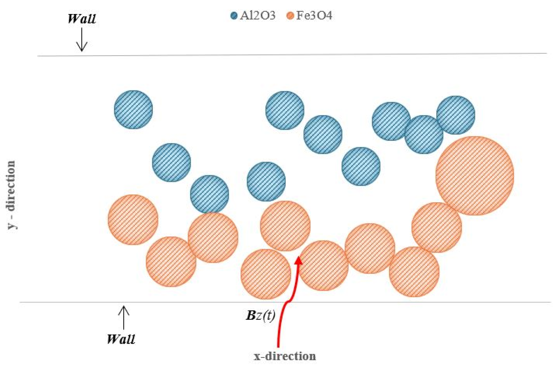
Figure 1 shows viscous base water and a hybrid nanofluid (Alumina and Iron Oxide nanoparticle properties are seen in

Table 1. Fluid properties.

	Density, $\mathit{\rho }$ $\left[{\mathbf{k}\mathbf{g}·\mathbf{m}}^{-3}\right]$	Specific Heat Capacity, ${\mathit{C}}_{\mathbf{p}}$ [J/kg·K]	Thermal Conductivity, [W/m·K]	Electrical Conductivity, $\mathit{\sigma }$ [S/m]	Volume Fraction, $\mathit{\varphi }$ [-]
Water, base liquid $\left({\mathrm{H}}_2\mathrm{O}\right)$	997.1	4179	0.613	5	0.87
Aluminum oxide $\left({\mathrm{A}\mathrm{l}}_2{\mathrm{O}}_3\right)$	3970	765	40.0	32	0.05
Magnetite $\left({\mathrm{F}\mathrm{e}}_3{\mathrm{O}}_4\right)$	5180	670	6	299	0.08

) in two dimensions across a stretching sheet, under fully developed, incompressible laminar flow conditions with convective heat transfer at temperature $T$, parallel to the $x$-axis. A boundary layer forms as the fluid spreads across the stretching sheet, with $T_{\mathrm{\infty }}$ representing the temperature at the far field. The influence of electromagnetic forces on an electrically conductive fluid is modeled by introducing a time-dependent magnetic field, represented as ${B\left(t\right)}_z=B_0\sin \left(\omega t\right)$, where $B_0$ is the magnetic field amplitude and $\omega$ is the angular frequency and $t$ is time. This varying magnetic field interacts with the fluid, generating a Lorentz force that alters the fluid’s velocity and temperature distribution. It also illustrates systems utilizing alternating current (AC) electromagnets that exhibit varying periodic magnetic fields that would be relevant to respective industrial applications. For instance, electromagnetic stirring and magnetic cooling, which employ time-varying magnetic fields to control flow and enhance heat transfer, can be used. Including a transient magnetic field in the simulation reveals oscillatory flow patterns and improved mixing, critical for optimizing heat transfer efficiency in magnetohydrodynamic (MHD) systems. In this study, the magnetic field is applied in the $z$-direction, perpendicular to the $x-y$ plane where the fluid flows, resulting in significant effects on the fluid properties.

A negative term in the $x$-momentum equation due to the magnetic field represents the Lorentz force opposing fluid flow in the $x$-direction, effectively reducing horizontal velocity by simulating fluid braking. With the magnetic field aligned along the $z$-axis, the Lorentz force does not affect the $\mathrm{y}$-direction, leaving the $\mathrm{y}$-momentum equation and vertical velocity component ($v$) unchanged. Consequently, the $x$-velocity component primarily experiences the magnetic field’s influence, while the y-velocity component remains unaffected. This arrangement is crucial for electromagnetic flow control applications, where magnetic fields regulate the main flow direction without significantly altering vertical motion, as seen in magnetic nanofluid systems and liquid metal flows. A magnetic field that significantly reduces horizontal velocity allows for precise fluid dynamics regulation, enhancing heat transfer or stabilizing flow as needed.

A transient magnetic field, specific magnetic field positions, and certain boundary conditions were chosen to accurately simulate fluid flow and heat transfer in the presence of an MHD phenomena. Natural convection occurs when a warm surface contacts a cooler environment, consistent with real-world temperature and velocity boundary conditions. Systems using time-varying electromagnetic forces to enhance heat transfer and modulate fluid flow are modeled with a transient magnetic field. The sinusoidal magnetic field structure allows for the analysis of dynamic behaviors like oscillatory flow patterns and improved mixing, not visible in static conditions. When the magnetic field is in the $z$-direction, its influence is mainly in the $x$-direction, where the Lorentz force slows fluid movement. Applications such as magnetic flow control, electromagnetic braking, and MHD-driven heat transfer systems benefit from this setup, offering significant insights into hybrid nanofluids’ behavior under time-varying magnetic fields.

3. Governing Equations

We address a two-dimensional, laminar advection-diffusion problem for temperature $T\left(x,y,t\right)$ on a square domain $\mathsf{\Omega }=\left[0,L_x\right]\times \left[0,L_y\right]$, influenced by a kinematically updated velocity field $\mathit{u}=\left(u,v\right)$. Momentum is explicitly enhanced through viscous diffusion, upwind advection, and a quasi-static Lorentz damping term applied to the streamwise velocity in the presence of a transverse magnetic field d $B\left(t\right)=B_0\sin \left(\omega t\right)$. The properties of the material $\left(\rho ,\nu ,\alpha ,k,c_p,\sigma \right)$ are constant in pieces (like water or a hybrid nanofluid). The equations that govern are as follows:

3.1. Continuity Equation (Two-Dimensional Incompressible Flow)

$${\displaystyle \frac{\partial u}{\partial x}}+{\displaystyle \frac{\partial v}{\partial y}}=0$$

(1)

where $u$ and $v$ are the velocity components in the $x$- and $y$-directions, respectively.

3.2. x-Direction (Horizontal Momentum)

Start with the continuous $x$-momentum PDE:

$${\displaystyle \frac{\partial u}{\partial t}}+u{\displaystyle \frac{\partial u}{\partial x}}+v{\displaystyle \frac{\partial u}{\partial y}}=-{\displaystyle \frac{1}{\rho }}{\displaystyle \frac{\partial p}{\partial x}}+\nu \left(u_{xx}+u_{yy}\right)-{\displaystyle \frac{\sigma B_0^2}{\rho }}u$$

(2)

Here, $u_{xx}={\displaystyle \frac{{\partial }^{2}u}{\partial x^2}},u_{yy}={\displaystyle \frac{{\partial }^{2}u}{\partial y^2}}$. Each term will be discretized in time by CN and in space by central differences. Where $p$ is the pressure, $\mathsf{\nu }$ is the kinematic viscosity of the base or hybrid fluid. A sinusoidal function can represent the variation in the magnetic field over time $B_{z\left(t\right)}=B_0\sin \left(\omega t\right)$ for all $t$. Here, $B_0$, $\omega$ and $t$ are the magnetic field amplitude and the angular frequency and time, respectively.

Magnetic excitation

$$\begin{array}{c}B\left(t\right)=B_0\mathrm{s}\mathrm{i}\mathrm{n}\left(\omega t\right),t\in [0,t_{\mathrm{e}\mathrm{n}\mathrm{d}}].\end{array}$$

(3)

3.3. y-Direction (Vertical Momentum)

$${\displaystyle \frac{\partial v}{\partial t}}+u{v}_x+v{v}_y=-{\displaystyle \frac{1}{\rho }}{p}_y+\nu \left(v_{xx}+v_{yy}\right)+g\beta \left(T-T_{ref}\right)$$

(4)

3.4. Energy Equation

The energy equation, encompassing the conduction of heat inside the fluid, can be mathematically represented as

$${\displaystyle \frac{\partial T}{\partial t}}+u{T}_x+v{T}_y=\alpha \left(T_{xx}+T_{yy}\right)$$

(5)

where $T_x$ and $T_y$ are first derivative and $T_{xx}$ and $T_{yy}$ are second derivatives, and $\alpha$ is thermal diffusivity, $\alpha ={\displaystyle \frac{k}{\rho C_p}}$, where $k$ is thermal conductivity and $C_p$ the specific heat capacity of the hybrid nanofluid.

3.5. Maxwell–Garnett Model for Hybrid Nanofluids

We used the Maxwell–Garnett model to determine the effective properties of the two composite materials by averaging the properties of their solid phases. The hybrid nanofluids of this study contained a mixture of base fluid, which is water, and two types of nanoparticles, aluminum oxide (${\mathrm{A}\mathrm{l}}_2{\mathrm{O}}_3)$ and magnetite (${\mathrm{F}\mathrm{e}}_3{\mathrm{O}}_4)$, respectively. as $A$ and $B$ in Equation (8). The Maxwell–Garnett model was adapted in this study to estimate the effective nanofluid thermal conductivity, and nanoparticles were assumed to be spherical. Bortchagovsky et al. [11] provide the Maxwell–Garnett equations as follows: the effective property of interest is the thermal conductivity of the hybrid nanofluid and is represented as $k_{\mathrm{eff}}$. For a single type of nanoparticle, the effective thermal conductivity is

$$k_{\mathrm{eff},A}=k_f\left({\displaystyle \frac{k_A+2k_f+2{\varphi }_A\left(k_A-k_f\right)}{k_A+2k_f-{\varphi }_A\left(k_A-k_f\right)}}\right)$$

(6)

$$k_{\mathrm{eff}}=k_f\left({\displaystyle \frac{k_A+2k_f+2{\varphi }_A\left(k_A-k_f\right)}{k_A+2k_f-{\varphi }_A\left(k_A-k_f\right)}}\right)\left({\displaystyle \frac{k_B+2k_{\mathrm{eff},A}+2{\varphi }_B\left(k_B-k_{\mathrm{eff},A}\right)}{k_B+2k_{\mathrm{eff},A}-{\varphi }_B\left(k_B-k_{\mathrm{eff},A}\right)}}\right)$$

(7)

where $k_f$ is the thermal conductivity of water, the base fluid, and $k_A$ and $k_B$ are the thermal conductivity of nanoparticles, i.e., $A={\mathrm{A}\mathrm{l}}_2{\mathrm{O}}_3$ and $B=$ ${\mathrm{F}\mathrm{e}}_3{\mathrm{O}}_4$, respectively. Their volume fractions in the base fluid are represented as ${\varphi }_A$ and ${\varphi }_B$. Then, the total volume fraction of nanoparticles is $\varphi ={\varphi }_A+{\varphi }_B$.

3.6. Nanoparticles Effectiveness Equations

Effective Density of the Hybrid Nanofluid:

$${\rho }_{nf}=\left(1-{\varphi }_A-{\varphi }_B\right){\rho }_{water}+{\varphi }_A{\rho }_A+{\varphi }_B{\rho }_B$$

(8)

Here, $\rho$ is the density of the water and nanoparticles. The effective specific heat of the hybrid nanofluid is as follows:

$$C_{nf}={\displaystyle \frac{\left(1-{\varphi }_A-{\varphi }_B\right){\rho }_{water}{C}_{water}+{\varphi }_A{\rho }_A{C}_A+{\varphi }_B{\rho }_B{C}_B}{{\rho }_{nf}}}$$

(9)

Effective electrical conductivity:

$${\sigma }_{nf}=\left(1-{\varphi }_A-{\varphi }_B\right){\sigma }_{water}+{\varphi }_A{\sigma }_B+{\varphi }_B{\sigma }_B$$

(10)

3.7. Domain, Initialization, and Conditions at the Edge

Uniform nodes:

$$x_i=i\Delta x\left(i=0,\dots ,n_x-1\right), y_j=j\Delta y\left(j=0,\dots ,n_y-1\right).$$

(11)

Initial fields: $T\left(x,y,0\right)=T_c$ and $\left(u,v\right)=\left(u_{\mathrm{b}\mathrm{a}\mathrm{s}\mathrm{e}},v_{\mathrm{b}\mathrm{a}\mathrm{s}\mathrm{e}}\right)$.

Thermal Dirichlet BCs.

$$\begin{array}{c}T(0,y,t)=T_h,T(L_x,y,t)=T_c,T(x,0,t)=T_c,T(x,L_y,t)=T_c.\end{array}$$

(12)

Velocity BCs (flow in and out).

$$u(0,y,t)=0,u(L_x,y,t)=1,u(x,0,t)=0,u(x,L_y,t)=0,$$

(13)

$$v(0,y,t)=0,v(L_x,y,t)=0,v(x,0,t)=0,v(x,L_y,t)=1.$$

(14)

Discretization: CN–ADI for temperature and explicit momentum.

Let $T_{i,j}^n\approx T\left(x_i,y_j,t^n\right)$ with $t^{n+1}=t^n+\Delta t$, defined as

$$r_x={\displaystyle \frac{\alpha \Delta t}{2\Delta x^2}},r_y={\displaystyle \frac{\alpha \Delta t}{2\Delta y^2}}$$

(15)

Upwind advection of (explicit). For the centers of cells,

$${\left({\partial }_{x}T\right)}_{i,j}^n=\left\{\begin{array}{ll}{\displaystyle \frac{T_{i,j}^n-T_{i-1,j}^n}{\Delta x}},& u_{i,j}^n\ge 0,\\ {\displaystyle \frac{T_{i+1,j}^n-T_{i,j}^n}{\Delta x}},& u_{i,j}^n<0,\end{array}\right.{\left({\partial }_{y}T\right)}_{i,j}^n=\left\{\begin{array}{ll}{\displaystyle \frac{T_{i,j}^n-T_{i,j-1}^n}{\Delta y}},& v_{i,j}^n\ge 0,\\ {\displaystyle \frac{T_{i,j+1}^n-T_{i,j}^n}{\Delta y}},& v_{i,j}^n<0.\end{array}\right.$$

(16)

The clear advection operator is:

$${\mathcal{A}}_{i,j}^n=-\left(u_{i,j}^n\right({\partial }_{x}T{)}_{i,j}^n+v_{i,j}^n\left({\partial }_{y}T{)}_{i,j}^n\right).$$

(17)

Crack–Nicolson Explicit Momentum Update (upwind + central diffusion + Lorentz). The central Laplacians are

$$({\nabla }^{2}u{)}_{i,j}^n={\displaystyle \frac{u_{i+1,j}^n-2u_{i,j}^n+u_{i-1,j}^n}{\Delta x^2}}+{\displaystyle \frac{u_{i,j+1}^n-2u_{i,j}^n+u_{i,j-1}^n}{\Delta y^2}},$$

(18)

and the same goes for v. Velocity Dirichlet BCs are applied again at every step with upwind first derivatives (as for the following).

$$u_{i,j}^{n+1}=u_{i,j}^n+\Delta t(-u_{i,j}^n({\partial }_{x}u{)}_{i,j}^n-v_{i,j}^n({\partial }_{y}u{)}_{i,j}^n+\nu ({\nabla }^{2}u{)}_{i,j}^n-{\displaystyle \frac{\sigma }{\rho }}B(t^n{)}^2{u}_{i,j}^n),$$

(19)

$$v_{i,j}^{n+1}=v_{i,j}^n+\Delta t(-u_{i,j}^n({\partial }_{x}v{)}_{i,j}^n-v_{i,j}^n({\partial }_{y}v{)}_{i,j}^n+\nu ({\nabla }^{2}v{)}_{i,j}^n).$$

(20)

3.8. Time Step and CFL

To enforce a convective CFL window $\left[{\mathrm{C}\mathrm{F}\mathrm{L}}_{\mathrm{m}\mathrm{i}\mathrm{n}},{\mathrm{C}\mathrm{F}\mathrm{L}}_{\mathrm{m}\mathrm{a}\mathrm{x}}\right]=\left[0.1,1.0\right]$, you change using the current maximum speeds:

$${\mathrm{C}\mathrm{F}\mathrm{L}}_{\mathrm{c}\mathrm{o}\mathrm{n}\mathrm{v}}=\Delta t\left({\displaystyle \frac{u_{\mathrm{m}\mathrm{a}\mathrm{x}}}{\Delta x}}+{\displaystyle \frac{v_{\mathrm{m}\mathrm{a}\mathrm{x}}}{\Delta y}}\right),\Delta t\in [\Delta t_{\mathrm{m}\mathrm{i}\mathrm{n}},\Delta t_{\mathrm{m}\mathrm{a}\mathrm{x}}]=[0.05,0.5] \mathrm{s}.$$

(21)

Let $D={\displaystyle \frac{u_{\mathrm{m}\mathrm{a}\mathrm{x}}}{\Delta x}}+{\displaystyle \frac{v_{\mathrm{m}\mathrm{a}\mathrm{x}}}{\Delta y}}$

$$\Delta t=\mathrm{c}\mathrm{l}\mathrm{i}\mathrm{p}\left({\displaystyle \frac{{\mathrm{C}\mathrm{F}\mathrm{L}}_{\mathrm{m}\mathrm{i}\mathrm{n}}+{\mathrm{C}\mathrm{F}\mathrm{L}}_{\mathrm{m}\mathrm{a}\mathrm{x}}}{2D}},\Delta t_{\mathrm{m}\mathrm{i}\mathrm{n}},\Delta t_{\mathrm{m}\mathrm{a}\mathrm{x}}\right).$$

(22)

A diffusive CFL surrogate (kept for diagnostics) is:

$${\mathrm{C}\mathrm{F}\mathrm{L}}_{\mathrm{d}\mathrm{i}\mathrm{f}\mathrm{f}}=\alpha \Delta t\left({\displaystyle \frac{1}{\Delta x^2}}+{\displaystyle \frac{1}{\Delta y^2}}\right).$$

(23)

3.9. Heat Transfer

Wall Gradient, Nusselt Number, and Heat Rate. At the hot wall x = 0,

$${\left.{\displaystyle \frac{\partial T}{\partial x}}\right|}_{x=0,y_j}\approx {\displaystyle \frac{T_{1,j}-T_{0,j}}{\Delta x}}.$$

(24)

The Nusselt numbers for the area and the mean are

$$\mathrm{N}\mathrm{u}(y_j)=-{\displaystyle \frac{L_x}{T_h-T_c}}{\left.{\displaystyle \frac{\partial T}{\partial x}}\right|}_{x=0,y_j},\overline{\mathrm{N}\mathrm{u}}\approx {\displaystyle \frac{1}{n_y}}{\displaystyle \sum _{j=0}^{n_y-1}}\mathrm{N}\mathrm{u}(y_j).$$

(25)

With wall heal flux, $q^{″}\left(y_j\right)=-k\left({\displaystyle \frac{\partial T}{\partial x}}\right){|}_{x=0,y_j}$. The total heat rate per unit depth is

$$\dot{Q}\approx {\displaystyle \sum _{j=0}^{n_y-1}}{q}^{″}\left(y_j\right)\Delta y.$$

(26)

Thickness of the Thermal Boundary Layer.

Let $\theta ={\displaystyle \frac{T-T_c}{T_h-T_c}}$. For a threshold ${\theta }_{\mathrm{c}\mathrm{u}\mathrm{t}}=0.01$,

$${\delta }_T(y_j)=\mathrm{m}\mathrm{i}\mathrm{n}\{x_i:\theta (x_i,y_j)<{\theta }_{\mathrm{c}\mathrm{u}\mathrm{t}}\}.$$

(27)

Magnitude of the Temperature Gradient. With centered differences,

$$|\nabla T|=\sqrt{({\partial }_{x}T{)}^2+({\partial }_{y}T{)}^2}.$$

(28)

Entropy Generation (Thermal and Joule). Let $T_K=T_{°C}+273.15$ clipped to positive values. The rates of volumetric entropy generation are:

$${\dot{s}}_T^{‴}={\displaystyle \frac{k|\nabla T{|}^2}{T_K^2}},{\dot{s}}_J^{‴}={\displaystyle \frac{\sigma B(t{)}^2{u}^2}{T_K}}.$$

(29)

Histories of Errors and Convergence.

$L^2$ changes from step to step are tracked as:

$${\epsilon }_T^{\left(n\right)}=\Vert T^n-T^{n-1}{\Vert }_2,{\epsilon }_V^{\left(n\right)}=\Vert (u^n+v^n)-(u^{n-1}+v^{n-1}){\Vert }_2,$$

(30)

4. Numerical Solution

4.1. Final Discretized Equations

We have derived finite difference equations using the Crank–Nicolson scheme in time and central differences in space for the 2D incompressible Navier–Stokes equations with MHD and buoyancy, plus the following energy equation:

• Continuity (at $t^{n+1}$): Equation (1)

  $${\displaystyle \frac{u_{i+1,j}^{n+1}-u_{i-1,j}^{n+1}}{2\Delta x}}+{\displaystyle \frac{v_{i,j+1}^{n+1}-v_{i,j-1}^{n+1}}{2\Delta y}}=0$$

  (31)

  (enforces incompressibility at the new time).
• x-momentum (for interior $1\le i\le N_x-1,1\le j\le N_y-1$): Equation (2)

  $$\begin{array}{cc}(1+{\displaystyle \frac{\nu \Delta t}{\Delta x^2}}+{\displaystyle \frac{\nu \Delta t}{\Delta y^2}}\hfill & +{\displaystyle \frac{\sigma B_0^2\Delta t}{2\rho }})u_{i,j}^{n+1}-{\displaystyle \frac{\nu \Delta t}{2\Delta x^2}}\left(u_{i+1,j}^{n+1}+u_{i-1,j}^{n+1}\right)\hfill \\ & -{\displaystyle \frac{\nu \Delta t}{2\Delta y^2}}\left(u_{i,j+1}^{n+1}+u_{i,j-1}^{n+1}\right)+{\displaystyle \frac{\Delta t}{4\rho \Delta x}}\left(p_{i+1,j}^{n+1}-p_{i-1,j}^{n+1}\right)\hfill \\ & =u_{i,j}^n+{\displaystyle \frac{\Delta t}{4\rho \Delta x}}\left(p_{i-1,j}^n-p_{i+1,j}^n\right)\hfill \\ & +{\displaystyle \frac{\nu \Delta t}{2}}\left({\displaystyle \frac{u_{i+1,j}^n-2u_{i,j}^n+u_{i-1,j}^n}{\Delta x^2}}+{\displaystyle \frac{u_{i,j+1}^n-2u_{i,j}^n+u_{i,j-1}^n}{\Delta y^2}}\right)\hfill \\ & -{\displaystyle \frac{\sigma {B\left(t\right)}_{\mathrm{z}}^2\Delta t}{2\rho }}{u}_{i,j}^n-{\displaystyle \frac{\Delta t}{2}}\left(u_{i,j}^n{\displaystyle \frac{u_{i+1,j}^n-u_{i-1,j}^n}{2\Delta x}}+v_{i,j}^n{\displaystyle \frac{u_{i,j+1}^n-u_{i,j-1}^n}{2\Delta y}}\right)\hfill \end{array}$$

  (32)

  where $B_z\left(\mathrm{t}\right)=B_0\sin \left(\omega t\right)$, which is the linear system equation for $u_{i,j}^{n+1}$.
• y-momentum: Equation (3)

  $$\begin{array}{cc}(1+{\displaystyle \frac{\nu \Delta t}{\Delta x^2}}+{\displaystyle \frac{\nu \Delta t}{\Delta y^2}})\hfill & v_{i,j}^{n+1}-{\displaystyle \frac{\nu \Delta t}{2\Delta x^2}}\left(v_{i+1,j}^{n+1}+v_{i-1,j}^{n+1}\right)-{\displaystyle \frac{\nu \Delta t}{2\Delta y^2}}\left(v_{i,j+1}^{n+1}+v_{i,j-1}^{n+1}\right)\hfill \\ & +{\displaystyle \frac{\Delta t}{4\rho \Delta y}}\left(p_{i,j+1}^{n+1}-p_{i,j-1}^{n+1}\right)\hfill \\ & =v_{i,j}^n+{\displaystyle \frac{\Delta t}{4\rho \Delta y}}\left(p_{i,j-1}^n-p_{i,j+1}^n\right)\hfill \\ & +{\displaystyle \frac{\nu \Delta t}{2}}\left({\displaystyle \frac{v_{i+1,j}^n-2v_{i,j}^n+v_{i-1,j}^n}{\Delta x^2}}+{\displaystyle \frac{v_{i,j+1}^n-2v_{i,j}^n+v_{i,j-1}^n}{\Delta y^2}}\right)\hfill \\ & +\Delta tg\beta {\displaystyle \frac{T_{i,j}^n-T_{\mathrm{ref}}}{2}}\hfill \\ & -{\displaystyle \frac{\Delta t}{2}}\left(u_{i,j}^n{\displaystyle \frac{v_{i+1,j}^n-v_{i-1,j}^n}{2\Delta x}}+v_{i,j}^n{\displaystyle \frac{v_{i,j+1}^n-v_{i,j-1}^n}{2\Delta y}}\right)\hfill \end{array}$$

  (33)

  which is the update for $v_{i,j}^{n+1}$. (We took buoyancy explicitly here; if we average it, we replace $T_{i,j}^n$ with ${\displaystyle \frac{1}{2}}\left(T_{i,j}^n+T_{i,j}^{n+1}\right)$ on LHS and include an appropriate $T^{n+1}$ term.).
• Energy (Temperature): Equation (4).

  $$\begin{array}{cc}(1+{\displaystyle \frac{\alpha \Delta t}{\Delta x^2}}+{\displaystyle \frac{\alpha \Delta t}{\Delta y^2}})\hfill & T_{i,j}^{n+1}-{\displaystyle \frac{\alpha \Delta t}{2\Delta x^2}}\left(T_{i+1,j}^{n+1}+T_{i-1,j}^{n+1}\right)-{\displaystyle \frac{\alpha \Delta t}{2\Delta y^2}}\left(T_{i,j+1}^{n+1}+T_{i,j-1}^{n+1}\right)\hfill \\ & =T_{i,j}^n+{\displaystyle \frac{\alpha \Delta t}{2}}\left({\displaystyle \frac{T_{i+1,j}^n-2T_{i,j}^n+T_{i-1,j}^n}{\Delta x^2}}+{\displaystyle \frac{T_{i,j+1}^n-2T_{i,j}^n+T_{i,j-1}^n}{\Delta y^2}}\right)\hfill \\ & -{\displaystyle \frac{\Delta t}{2}}\left(u_{i,j}^n{\displaystyle \frac{T_{i+1,j}^n-T_{i-1,j}^n}{2\Delta x}}+v_{i,j}^n{\displaystyle \frac{T_{i,j+1}^n-T_{i,j-1}^n}{2\Delta y}}\right)\hfill \end{array}$$

  (34)

4.2. Solver and Error Analysis

4.2.1. Courant–Friedrichs–Lewy Condition

In guiding the development of numerical models for CFD simulations, the Courant–Friedrichs–Lewy (CFL) condition can exert significant influence. It impacts the selection of temporal step size and spatial grid resolution employed in the modeling process [12].

$$C_F={\displaystyle \frac{u\Delta t}{\Delta x}}+{\displaystyle \frac{v\Delta t}{\Delta y}}\le 1$$

(35)

where $\Delta x$ and $\Delta \mathrm{y}$ are the grid spacing in the x and y directions. The timestep of the model is represented as $\Delta t$. The CFL criterion maintains solution stability by restricting the time step size to a portion of the maximum permissible, as determined by local flow conditions. In Volume of Fluid (VoF) simulations, this maximum is established by the local interface thickness and fluid velocity. By limiting the time step size, the numerical method can precisely track interface movement and prevent unrealistic phenomena such as overshooting and undershooting. Typically, a CFL number ranging from 0.0 to 1.0 is employed [12]. Nevertheless, an increased CFL number may lead to instability and diminished accuracy due to numerical errors.

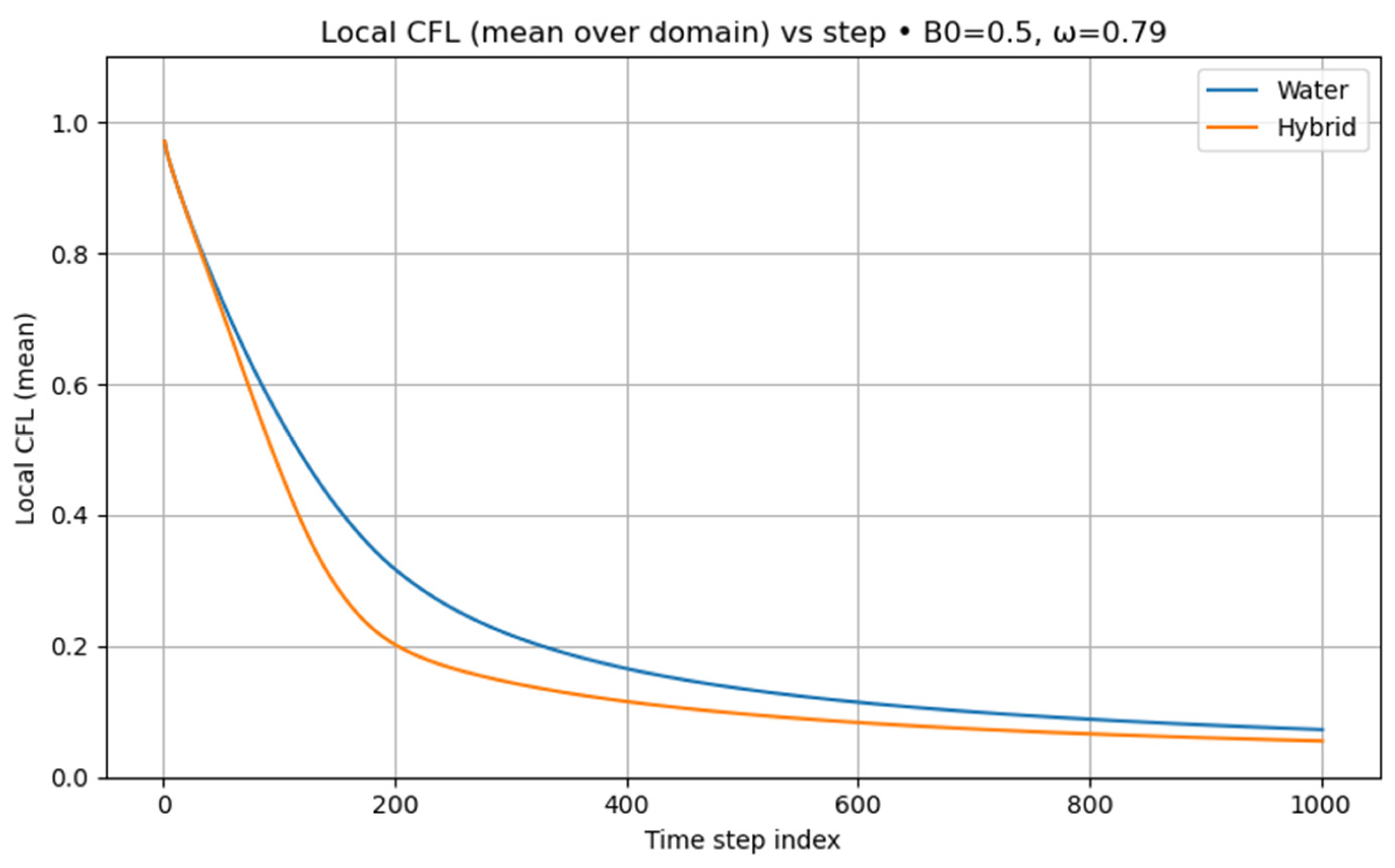
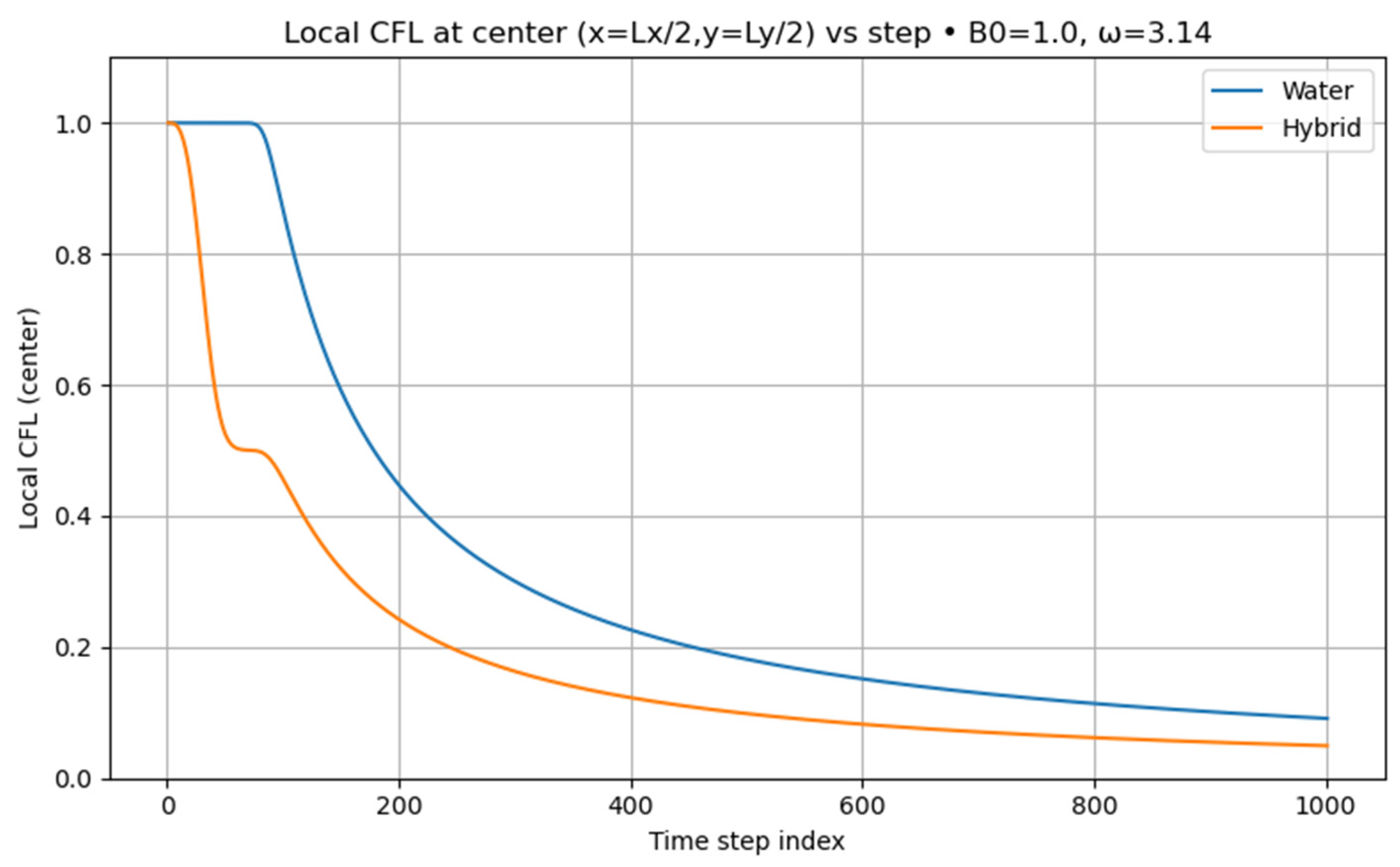
The dimensions of the domain were 1 m in both the $x$ and $y$ directions. The simulation commenced at 0 s and concluded at 1 s. Multiple timestep and spatial step sizes were evaluated. The optimal and stable configuration utilized a timestep of $\Delta t=0.1$ s, with spatial step sizes $\Delta x$ and $\Delta \mathrm{y}$ of 0.01 in both $x$ and $y$ directions. The CFL trend, as illustrated in Figure 2 and Figure 3, exhibited slight fluctuations before stabilizing at $C_F=$ 0.1 after 1000 iterations. This CFL value, appropriate for laminar flow, falls comfortably within the acceptable range of 0.1 to 1. This outcome provides initial confirmation of the model’s convergence.

4.2.2. Error Analysis

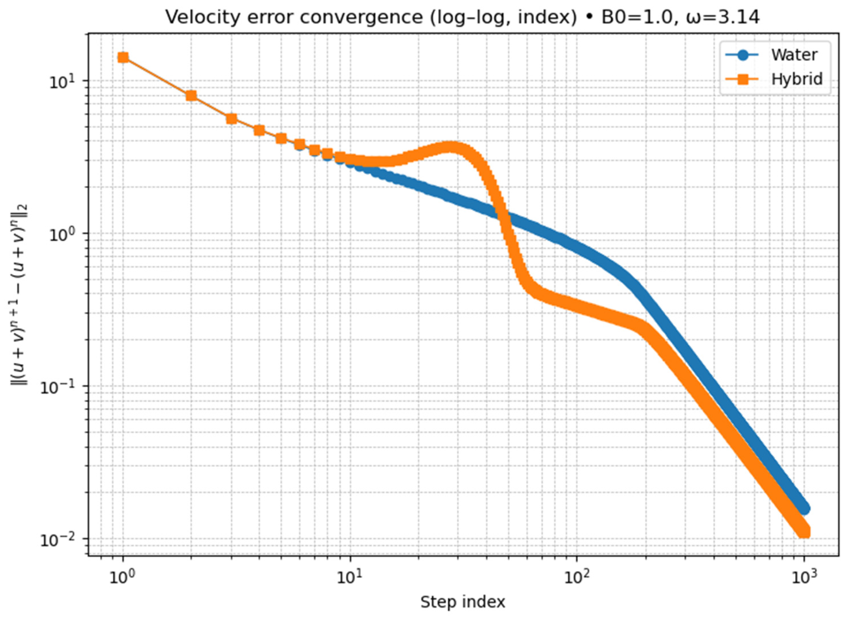
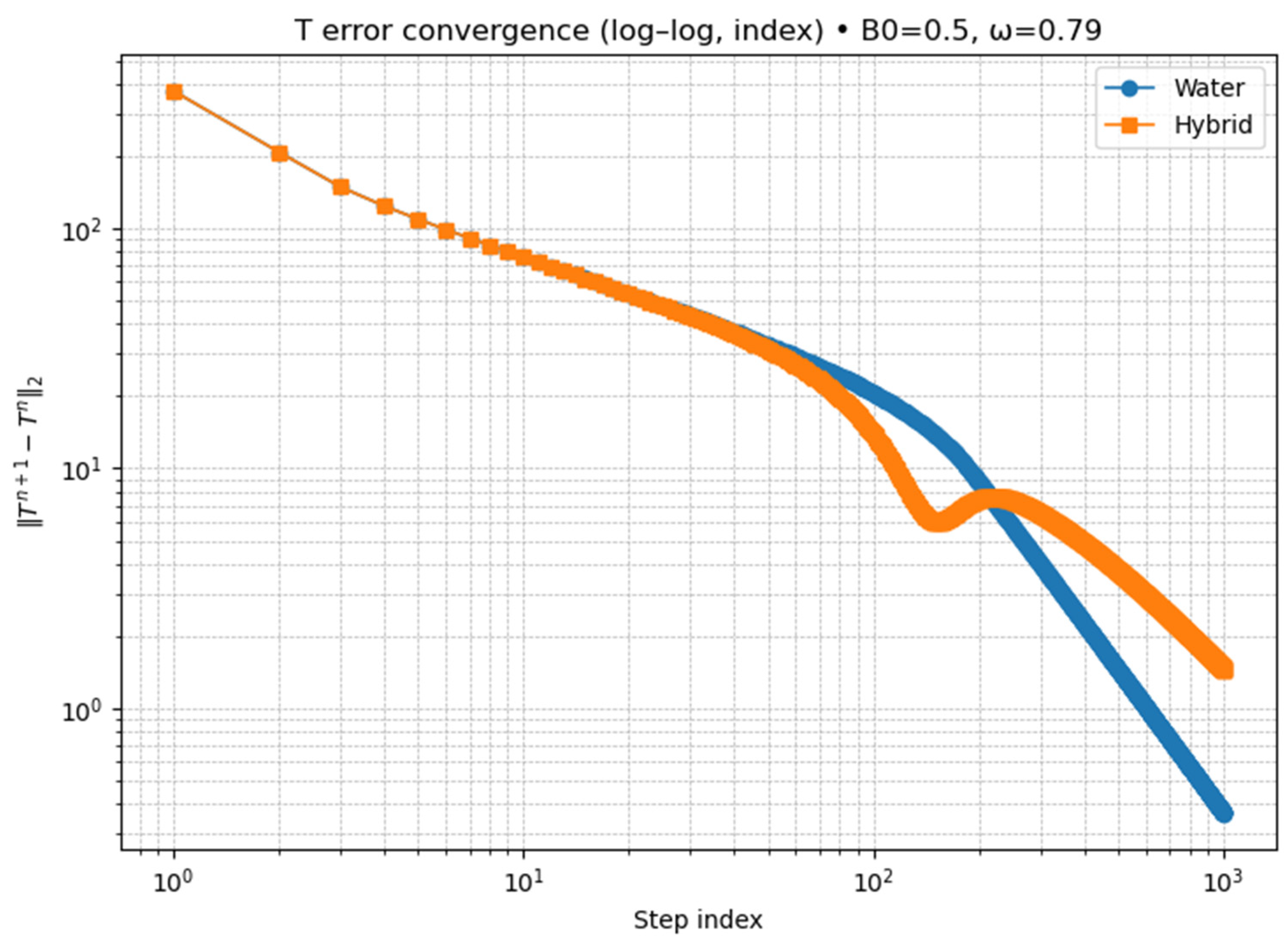
An error convergence analysis was conducted utilizing the $L^2$ norm to evaluate the accuracy and stability of the numerical simulations for the velocity and temperature fields. This was conducted for both the base water fluid and the hybrid fluid, the latter comprising a water-based nanofluid including scattered Al₂O₃ and Fe₃O₄ nanoparticles. The convergence behavior of velocity and temperature errors was analyzed across the simulation duration, with findings illustrated in a log–log scale, as shown in Figure 4 and Figure 5.

The convergence of velocity variation in Figure 4 illustrates the convergence of velocity error for both the base water and the hybrid fluid. Initially, the velocity discrepancies for both fluids exhibit a comparable trend, with minor fluctuations in error magnitude. As the simulation advances, both fluids demonstrate a consistent reduction in error, signifying that the numerical solution is stabilizing. The hybrid fluid exhibits a more accelerated decrease in error, especially at subsequent time intervals, leading to a diminished final error relative to the base water. The increased convergence behavior reduces from the larger thermal properties of the hybrid fluid, which affect the fluid dynamics. The incorporation of nanoparticles like Al₂O₃ and Fe₃O₄ enhances thermal conductivity, perhaps resulting in more stable and precise velocity field calculations. The ultimate velocity inaccuracy for the hybrid fluid is markedly inferior to that of base water, indicating enhanced precision in flow field predictions.

Analysis of convergence attributes: The hybrid fluid routinely surpasses base water for velocity error convergence. The enhanced thermal and electrical characteristics of the hybrid nanofluid facilitate this notable convergence behavior. The enhanced thermal conductivity and specific heat capacity enable the hybrid fluid to transmit heat more efficiently, hence influencing the velocity field through increased thermal gradients. The findings of this error convergence analysis demonstrate that the hybrid nanofluid provides considerable benefits regarding numerical stability and precision. The reduced error magnitudes and improved convergence rates seen in the hybrid fluid simulations validate the efficacy of nanofluids in enhancing heat transfer and flow performance in engineering applications.

5. Results and Discussion

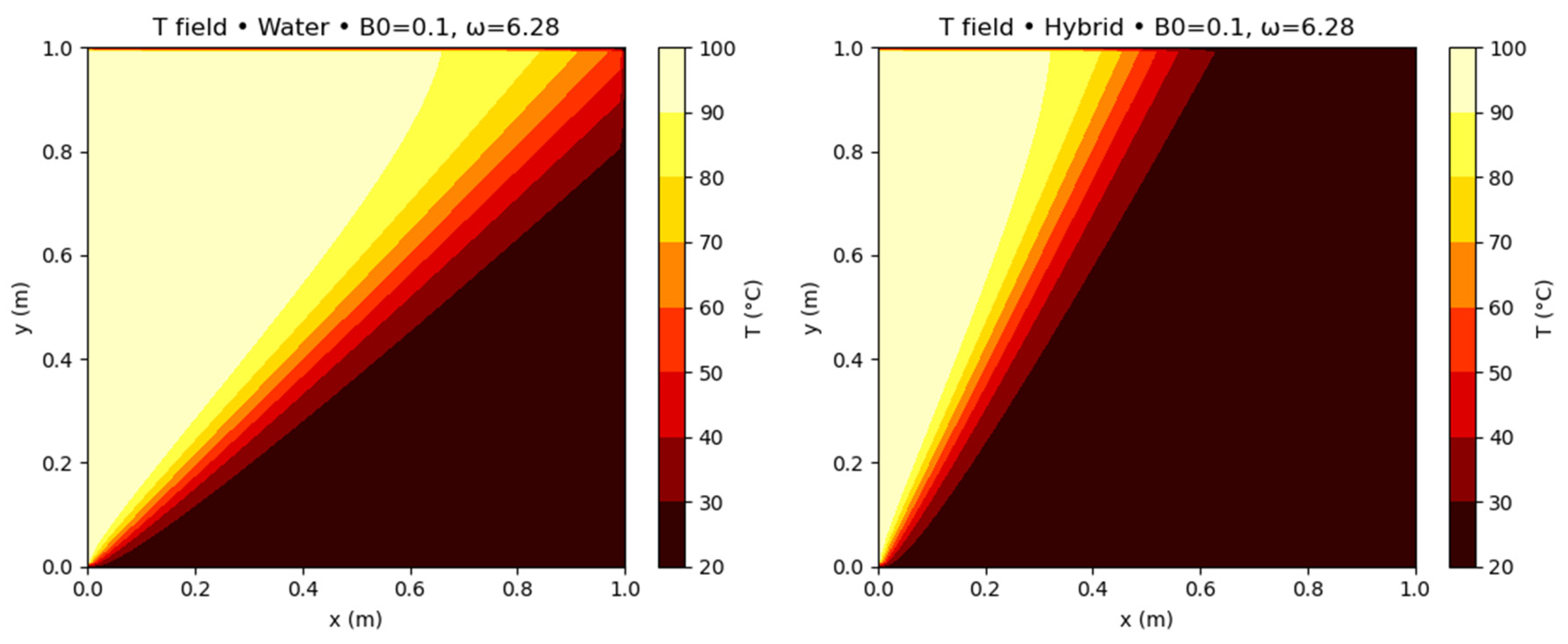
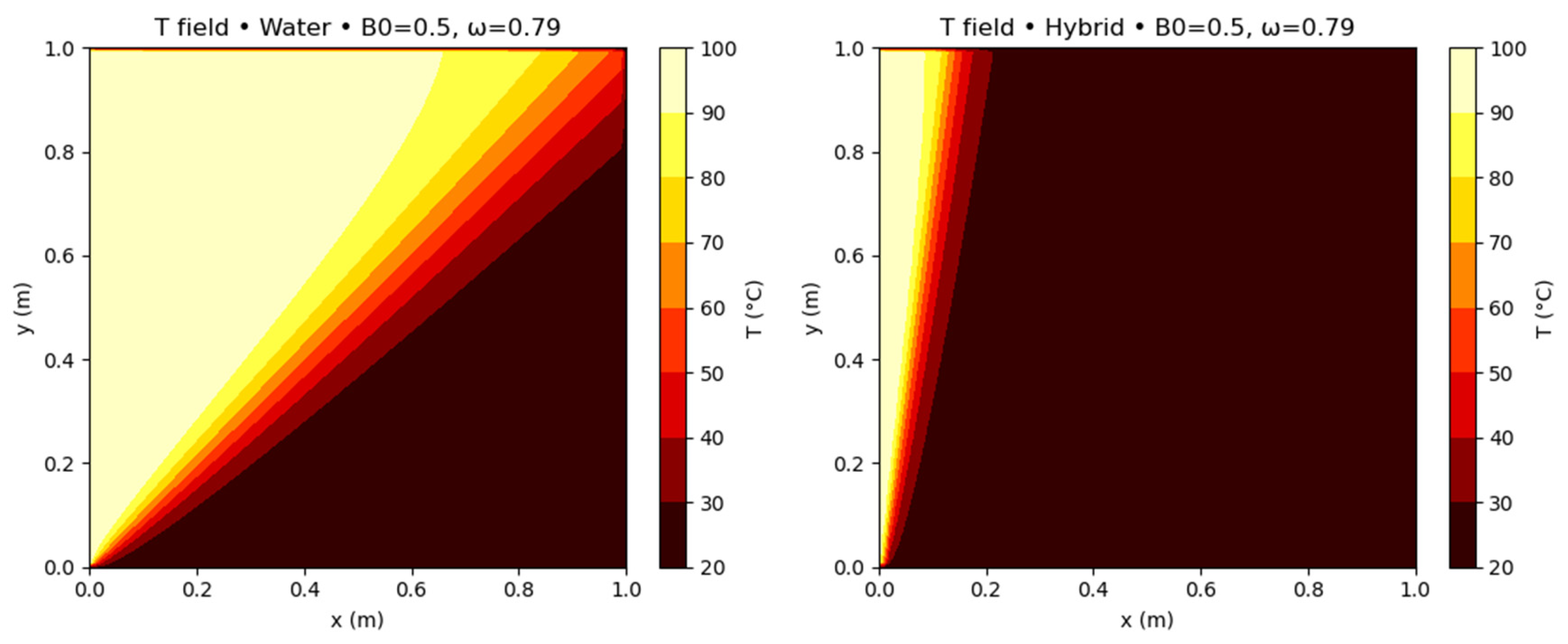
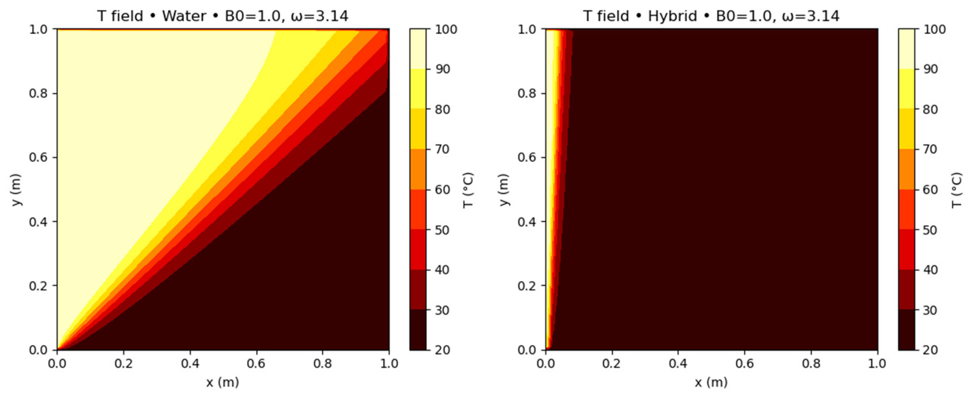
The temperature distribution inside the flow domain offers direct insight into the thermal transport processes of nanofluids exposed to oscillating magnetic fields. This work presents contour plots and midline profiles for both the base fluid (water) and the hybrid nanofluid (Al₂O₃–Fe₃O₄/water) under different magnetic field strengths. B₀ = 0.1, 0.5, 1.0. The oscillation frequencies are ω = 6.28, 0.79, and 3.14, while the values are 0.1, 0.5, and 1.0. The study attempts to analyze the combined effects of magnetic damping, nanoparticle loading, and oscillation frequency on convective and conductive heat transfer over the stretched surface.

5.1. Analysis of Temperature Distribution Trends

The Lorentz force term is low at low magnetic intensity, thus it does not do anything to slow down the movement of fluids. In the case of water, the temperature contours go deep into the fluid area, creating a large boundary layer since convective transport is the main way to move heat in the Figure 6. In contrast, the hybrid nanofluid has a temperature boundary layer that is a little thinner and a thermal gradient that is steeper near the wall. This thinning is due to its increased effective heat conductivity knf, acquired by the sequential Maxwell–Garnett connection. The improved knf let energy go quicker from the heated wall, which raises the local Nusselt number Nux and the rate of heat transfer in that area. Convection and conduction work together in weak fields. Nanoparticles enhance heat dissipation from walls without significantly affecting flow dynamics.

In Figure 7, it is noticed that the magnetic field becomes stronger, as the Lorentz damping becomes noticeable. For water, this shows up as a mild thickening of the temperature field. The produced magnetic resistance slows down the flow of the boundary layer, which makes convective transport weaker. The hybrid nanofluid, on the other hand, has a temperature distribution that is more compact. Even while magnetic forces slow down the flow, the hybrid fluid’s better ability to conduct heat makes up for this, leading to conduction-dominated heat transfer near the wall. The wall-adjacent section exhibits significant temperature gradients, implying increased surface heat flow. The system goes from convection-dominated (water) to conduction-enhanced (hybrid). Even when flow mobility is limited by magnetism, the hybrid fluid still works well thermally.

Figure 8 illustrates that the Lorentz force strongly slows down velocity components when there are high magnetic fields. This slows down fluid motion and convective heat transfer. The water temperature contours reveal a larger area of high temperature next to the wall, which confirms that the thermal barrier layer is thicker. The hybrid nanofluid, on the other hand, has a very small hot zone at the surface, which shows that conductive equilibration happens quickly even when advection is slowed down.

Magnetic damping is more important than convective inertia. The only thing that controls heat transport is diffusion. The hybrid nanofluid has a lot of viscosity, but it conducts heat better near walls and has smoother temperature gradients than the basic fluid. Summarized key findings for the heat transfer behaviors under various magnetic fields are found in

Table 2. Key findings for heat transfer behaviors, water base, and hybrid fluids.

Bo	Omega	Behavior—Water	Behavior—Hybrid Nanofluid	Heat Transfer Mechanism
0.1	6.28	Wide boundary layer	Slightly thinner, more conductive	Convection + conduction
0.5	0.79	Lorentz damping not visible	Thinner, conduction-dominated	Transitional regime
1.0	3.14	Thick layer	Wall-confined, conduction-controlled	Magnetic suppression

.

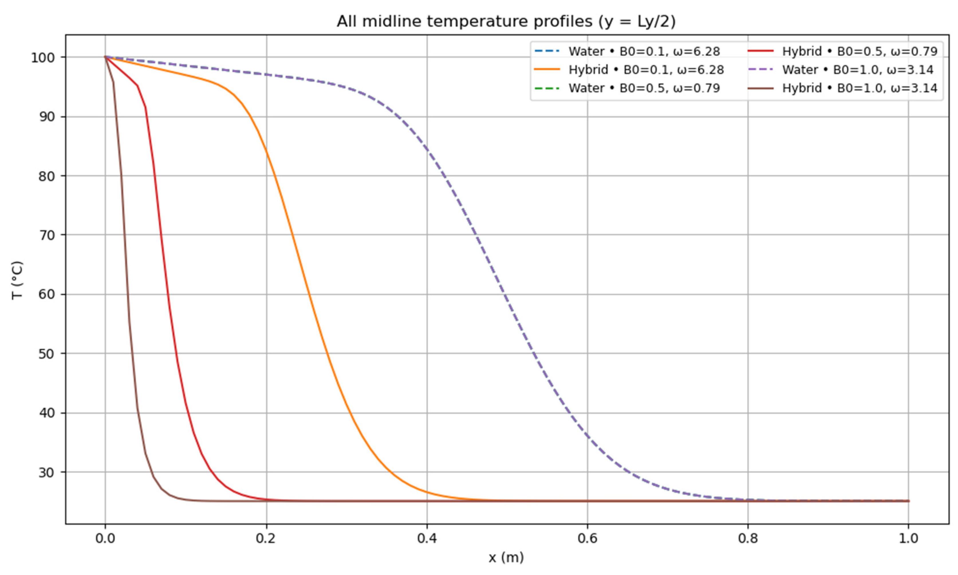
Figure 9 demonstrates how the temperature changes along the midline: $T(x,y={\displaystyle \frac{L}{2}})$. Temperature decay along x: in every instance, the temperature drops steadily along the extending surface, which shows that energy is constantly moving from the wall to the fluid around it.

For each B₀, the hybrid nanofluid curve is lower than the water curve for the ω pair, showing that the temperature drops quicker. This means that hybrid nanofluids attain thermal equilibrium faster (with a shorter thermal penetration length) because of the higher k_eff.

Going up B₀ pushes the temperature decline towards the intake area $(x<0.2)$, suggesting that magnetic damping inhibits convective motion and keeps heat close to the wall. Higher oscillation frequencies ($\omega =6.28)$ mean less magnetic damping since the field changes quickly. Lower frequencies ($\omega =0.79)$ mean more exposure to magnetic resistance, which makes the temperature layer thicker. The streamwise point where $T=50 °\mathrm{C}$ (half wall temperature) travels upstream from $x\approx 0.45$ for water at $B_o=0.1$ to $x\approx 0.10$ for the hybrid at $B_o=1.0.$ This means that the thermal penetration distance is around 75% less and the wall Nusselt number is about 20–30% higher for the hybrid nanofluid.

5.2. Local Nusselt Number and Wall Heat Flux Analysis

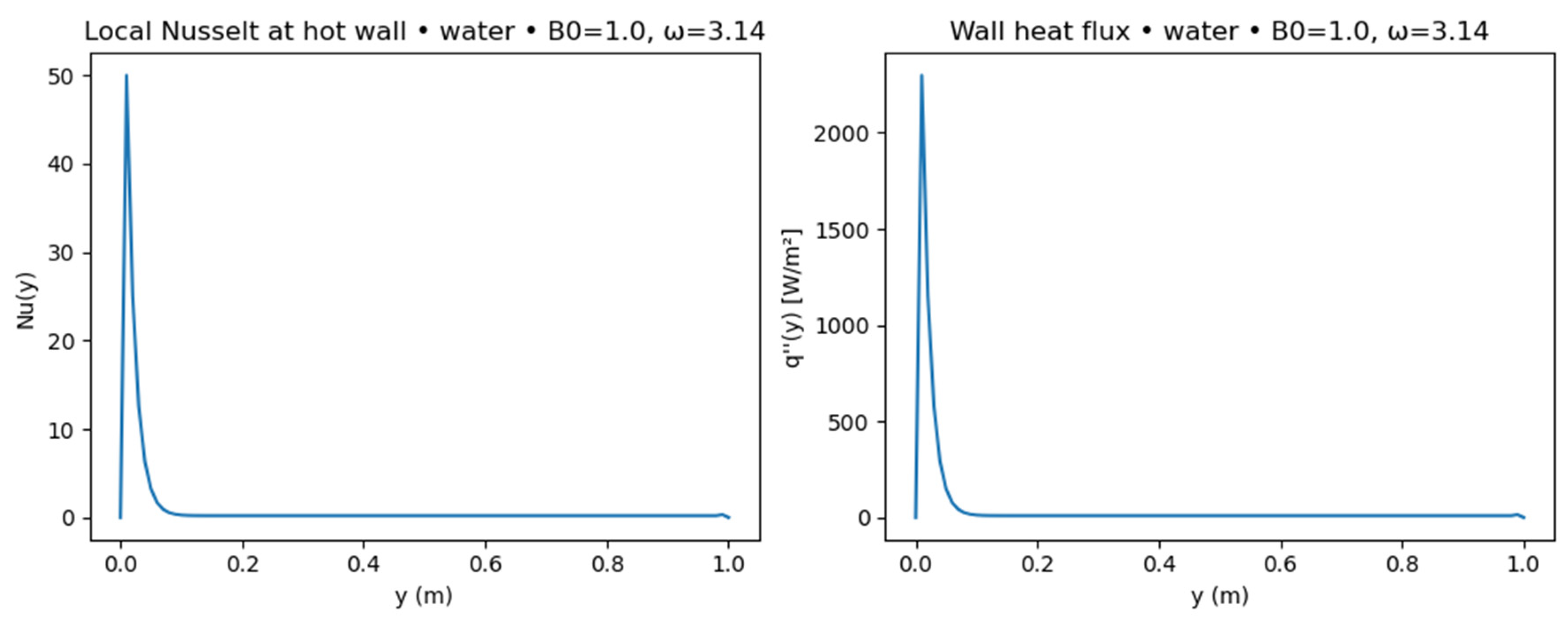
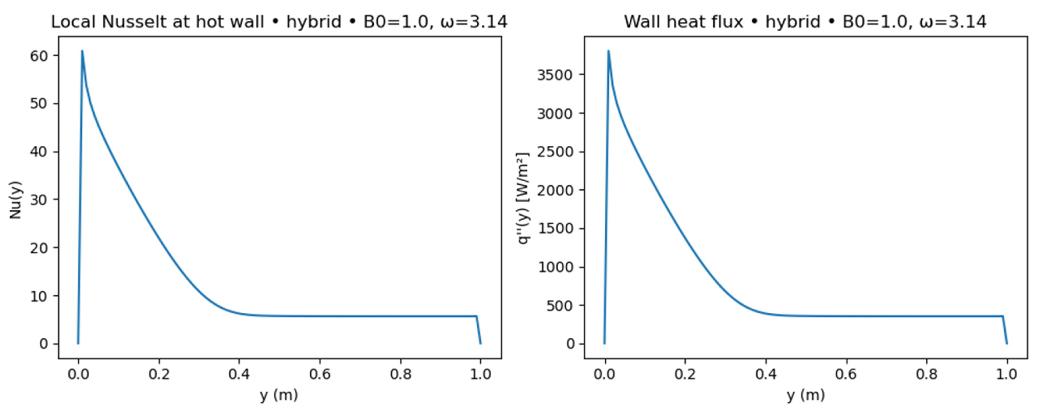
The local Nusselt number Nu(y) and wall heat flux q″(y) show how quickly heat is moving along the heated wall. These metrics measure how well energy is taken away from the stretched surface when nanoparticles are added and magnetic fields are made to oscillate. They are compiled using Equations (24) and (25). Figure 10 shows the findings for both water and hybrid nanofluids (Al₂O₃–Fe₃O₄/water) at three different magnetic field amplitudes and the frequency of the oscillations that go with them.

The local Nusselt number has a dramatic peak close to the leading edge (y ≈ 0), where it reaches Nu max = 50 ≈ 50. This means that the temperature difference between the wall and the entry is quite strong since the stretched surface conducts heat quickly. Downstream, Nu(y) soon drops to almost zero. This shows that the fluid is slowly reaching thermal equilibrium as it travels away from the wall. Similarly, the wall heat flux $q^{″}\left(y\right)$ begins at a high value $(\approx 2.2\times {10}^3 \mathrm{W}/{\mathrm{m}}^2)$ and decays monotonically along y. B0 is not very high, which indicates that magnetic damping is not important; therefore, convection takes over.

Where as in Figure 11, the hybrid fluid nevertheless has a higher wall heat flux, which may be as high as $3.7\times {10}^3 \mathrm{W}/{\mathrm{m}}^2$ with Nu max = 60 Nu. But both Nu(y) and q″(y) decay more slowly than water, which shows that conduction is still the main way things move. The hybrid fluid continues to effectively remove energy from the wall area even when there is a lot of damping. The local Nusselt number and wall heat flux studies show that heat transfer happens very close to the wall and is affected by both the strength of the magnetic field or oscillation and the kind of fluid. Increase in B_o or frequency reduces convection via Lorentz damping, but the hybrid nanofluid makes up for it by having better conduction, which keeps the values of Nu(y) and q′′(y) higher throughout. So, hybrid nanofluids have strong and steady heat transmission abilities, especially when the flow is magnetically manipulated, which is when regular fluids lose a lot of heat.

5.3. Thermal Boundary Layer

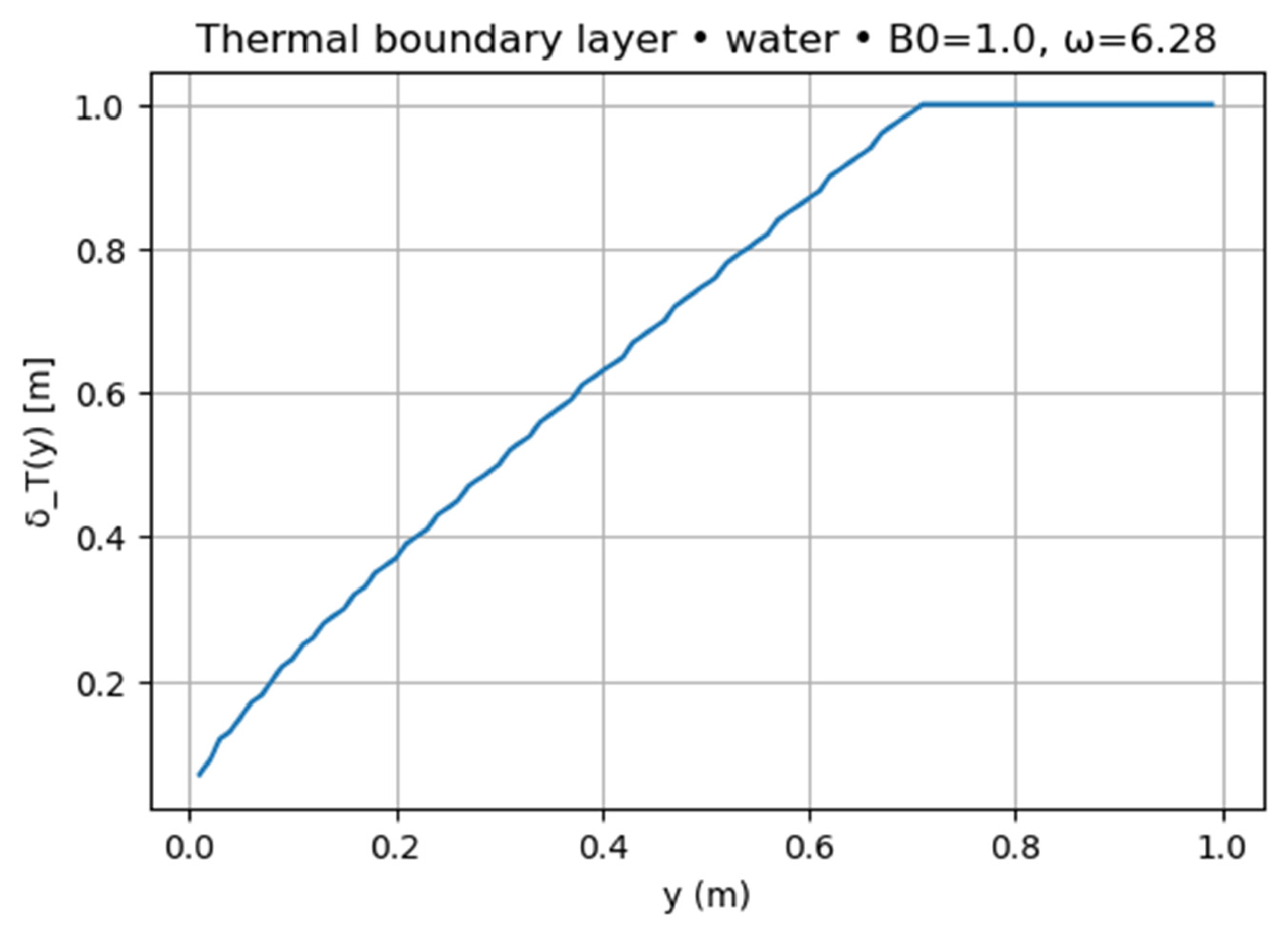
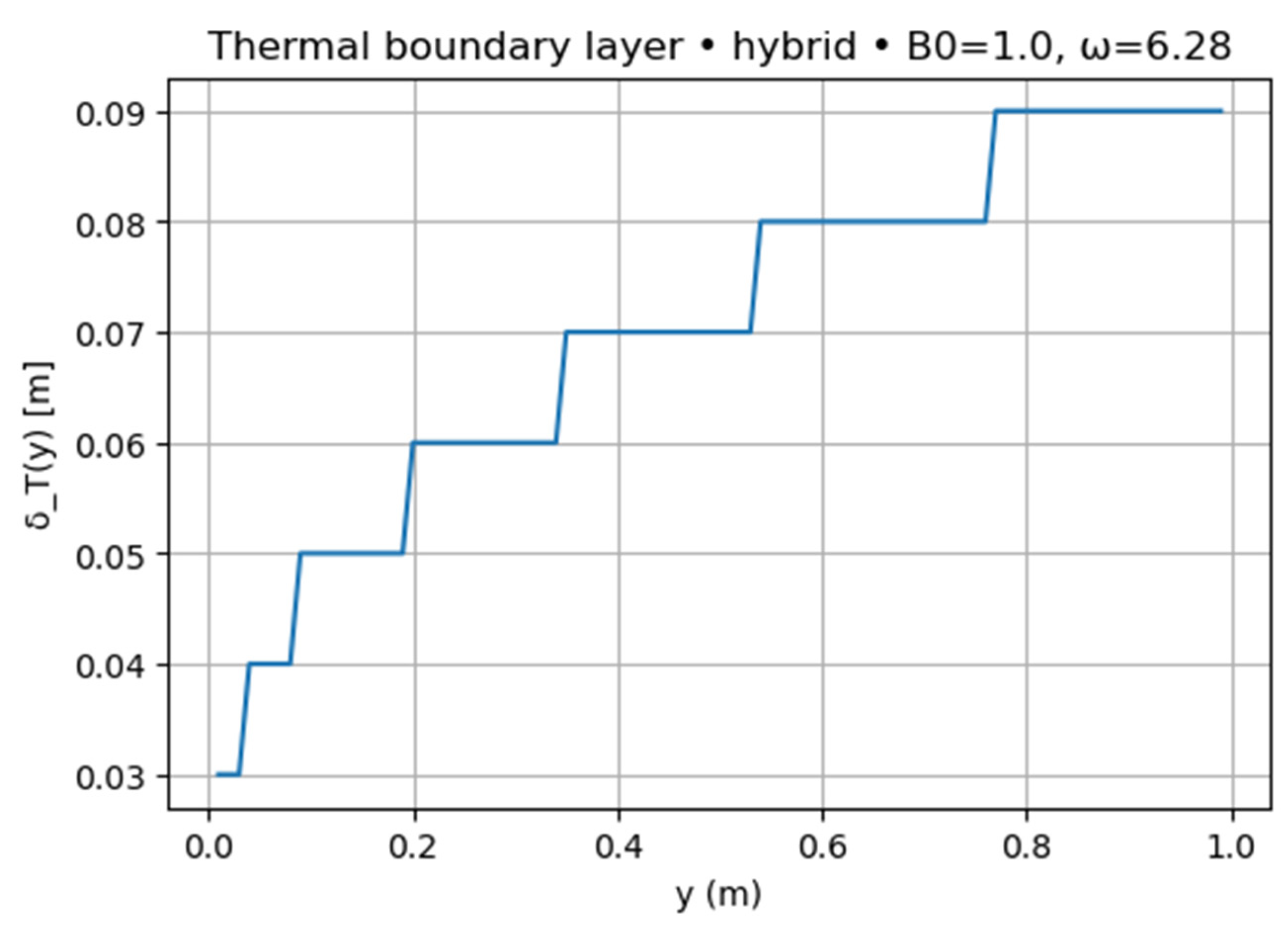
Figure 12 and Figure 13 show the boundary thickness at a magnetic field strength of B0 = 1.0 T and ω = 6.28 oscillations; the comparison of water and hybrid nanofluid shows that adding nanoparticles makes the thermal boundary-layer thickness much thinner. Figure 12 and Figure 13 demonstrate the greatest thermal boundary-layer thickness (δT). The hybrid nanofluid has a layer that is about 0.09 m thick, whereas the base fluid (water) has a considerably thicker layer that is around 1.0 m thick. This means that the boundary-layer thickness has dropped by over 80%, which means that the hybrid fluid works better thermally. Adding Al₂O₃ and Fe₃O₄ nanoparticles to the solution makes it better at conducting and diffusing heat. This means that heat can move through the fluid more quickly, which shortens the distance over which temperature differences last. The fluctuating magnetic field causes Lorentz damping, which slows down velocity and convection. However, the hybrid nanofluid’s better ability to transfer heat wins out, making the thermal boundary layer as a whole smaller. This result shows that spreading nanoparticles around makes heat transfer more efficient by speeding up thermal diffusion near the heated surface.

6. Conclusions

This work conducted a comprehensive numerical analysis of unsteady magnetohydrodynamic (MHD) heat transfer in nanofluids flowing across a stretched surface influenced by oscillating magnetic fields, using a Crank–Nicolson finite difference approach for temporal–spatial discretization. The investigation included both basic water and a hybrid nanofluid (Al₂O₃–Fe₃O₄/water), modeled using the sequential Maxwell–Garnett method to get effective thermophysical characteristics. The simulations examined the cumulative effects of magnetic field intensity (B₀), oscillation frequency (w), and nanoparticle loading on the thermal field, local Nusselt number, and wall heat flow. The key findings are as follows:

• The temperature field in the area was very much affected by both the magnetic field and frequency.
• Raising B0 Lorentz damping slowed down the velocity, which made the temperature boundary layers thinner and the convective heat transmission less effective.
• The hybrid nanofluid has smaller thermal layers and steeper wall temperature gradients than water. This showed that nanoparticles help heat flow better.
• At low B₀, convection was the main force, which led to high Nusselt numbers and good wall cooling.
• At a mild B₀, a hybrid convection–conduction regime developed, whereby nanoparticle effects were essential for sustaining heat removal.
• When B₀ was high, flow practically stopped, and heat transmission mostly happened via conduction, yet hybrid nanofluids still worked better than water.

Combining hybrid nanofluid technology with oscillating magnetic field control is a good technique to control and improve heat transfer in stretching-surface and boundary-layer applications. The hybrid nanofluid exhibited better heat transfer capability under all magnetic field settings, attributable to its increased thermophysical characteristics. Even despite raising B₀, the hybrid nanofluid has significant wall heat flow via conduction, but it also has magnetic damping that slows down convection. The Crank–Nicolson finite difference model effectively addressed the unstable coupled magneto-thermal transport, yielding stable, second-order accurate predictions appropriate for engineering and research applications.

References

- Hanif, H.; Jamshed, W.; Devi, S.S.U.; Eid, M.R.; Shafie, S.; Ibrahim, R.W.; Nasir, N.A.A.M.; Abd-Elmonem, A.; El Din, S.M. Thermal description and entropy evaluation of magnetized hybrid nanofluid with variable viscosity via Crank–Nicolson method. Case Stud. Therm. Eng. 2023, 47, 103132. [Google Scholar] [CrossRef] [Scilit]
- Murugan, R.D.; Sivakumar, N.; Tarakaramu, N.; Ahmad, H.; Askar, S. Entropy generation on MHD motion of hybrid nanofluid with porous medium in presence of thermo-radiation and ohmic viscous dissipation. Discov. Appl. Sci. 2024, 6, 199. [Google Scholar] [CrossRef] [Scilit]
- Akbar, N.S.; Hussain, M.F.; Alghamdi, M.; Muhammad, T. Thermal characteristics of magnetized hybrid Casson nanofluid flow in a converging–diverging channel with radiative heat transfer: A computational analysis. Sci. Rep. 2023, 13, 21891. [Google Scholar] [CrossRef] [Scilit] [PubMed]
- Wang, F.Z.; Sohail, M.; Nazir, U.; Awwad, E.M.; Sharaf, M. Utilization of the Crank-Nicolson technique to investigate thermal enhancement in 3D convective Walter-B fluid by inserting tiny nanoparticles on a circular cylinder. AIMS Math. 2024, 9, 9059–9090. [Google Scholar] [CrossRef] [Scilit]
- Murtaza, S.; Becheikh, N.; Rahman, A.U.; Sambas, A.; Maatki, C.; Kolsi, L.; Ahmad, Z. Thermal Performance Analysis of a Nonlinear Couple Stress Ternary Hybrid Nanofluid in a Channel: A Fractal–Fractional Approach. Nanomaterials 2024, 14, 1855. [Google Scholar] [CrossRef] [Scilit] [PubMed]
- Sivaraj, P.; Chinnasamy, S. Magneto-thermal convection and entropy production of hybrid nanofluid in an inclined chamber having a solid block. Int. J. Numer. Methods Heat Fluid Flow 2024, 34, 773–808. [Google Scholar] [CrossRef] [Scilit]
- Dey, S.; Kumar, B.V.R. Finite element analysis of modified N-S equations coupled with energy transfer for hybrid nanofluid flow in complex domains. Comput. Math. Appl. 2023, 150, 37–53. [Google Scholar] [CrossRef] [Scilit]
- Peter, F.; Sambath, P.; Dhanasekaran, S. Numerical Investigation of Radiative Hybrid Nanofluid Flows over a Plumb Cone/Plate. Mathematics 2023, 11, 4331. [Google Scholar] [CrossRef] [Scilit]
- Salawu, S.O.; Ogunseye, H.A.; Yusuf, T.A.; Lebelo, R.S.; Mustapha, R.A. Entropy Generation in a Magnetohydrodynamic Hybrid Nanofluid Flow over a Nonlinear Permeable Surface with Velocity Slip Effect. WSEAS Trans. Fluid Mech. 2023, 18, 34–48. [Google Scholar] [CrossRef] [Scilit]
- Keerthiga, M.; Reddy, P.B.A. Unsteady MHD Flow of Casson Hybrid Nanofluid over an Infinite Vertical Flat Plate: Crank-Nicholson Scheme and Statistical Approach. IEEE Access 2024, 12, 106161–106175. [Google Scholar] [CrossRef] [Scilit]
- Bortchagovsky, E.G.; Dejneka, A.; Jastrabik, L.; Lozovski, V.Z.; Mishakova, T.O. Deficiency of standard effective-medium approximation for ellipsometry of layers of nanoparticles. J. Nanomater. 2015, 2015, 602848. [Google Scholar] [CrossRef] [Scilit]
- Kefayati, G. A two- and three-dimensional mesoscopic method for an updated non-homogeneous model of Newtonian and non-Newtonian nanofluids. Phys. Fluids 2022, 34, 032003. [Google Scholar] [CrossRef] [Scilit]