Abstract
The use of different energy sources for heating and year-round domestic water heating is driven by the European Union’s increasingly strict environmental and climate requirements. For this reason, consumers are seeking alternatives and show growing interest in implementing installations that utilize solar energy. Modern households typically employ at least two different energy sources for this purpose. In practice, these are hybrid installations that, depending on the season, can operate with one, two, or more energy sources. The system examined in this paper is of this type, comprising a pellet boiler, solar vacuum tubes, and electric heaters. Managing such a system is complex, and based on the conducted studies, process optimization can be pursued. This report presents an artificial neural network (ANN) model developed to predict the behavior of a real solar installation for domestic hot water heating during the summer season. This study aims, through the obtained model, to forecast the system’s performance during transitional periods such as autumn and spring, thereby enabling more efficient control.
1. Introduction
The growing requirements of the European Union regarding the use of conventional heating methods, along with the promotion of new technologies, have led to a boom in the commissioning of systems employing diverse energy sources. This study is directly related to the current energy policies of the European Union, which aim to accelerate the deployment of renewable energy sources and improve overall energy efficiency. The European Green Deal and the ‘Fit for 55’ package set the ambitious target of achieving climate neutrality by 2050 and reducing greenhouse gas emissions by at least 55% by 2030. In this context, the use of solar systems for domestic hot water, combined with intelligent control methods based on artificial neural networks, represents a practical contribution to the implementation of the Energy Efficiency Directive (Directive (EU) 2023/1791) and the Renewable Energy Directive (RED III, Directive (EU) 2023/2413). On one side are boilers using biofuels, natural gas, or heat pumps that rely on various media as heat-transfer agents. These systems may produce some combustion by-products, albeit minimal, and they require periodic maintenance, while the initial investment is significant. Regardless of the energy source, electrical power is always used to control the overall system. On the other side are systems utilizing free solar energy, where the investment costs are lower, maintenance is cheaper, and they can operate year-round in practice.
Most heating and domestic hot water systems do not rely on a single energy source. By their nature, these systems are hybrid, allowing the use of multiple energy sources, which provides flexibility in operation. Various methods are applied to achieve higher system efficiency. The heating season is particularly important, with the greatest challenge occurring in the spring and autumn transitional periods, where process optimization can be realized. Data collected from a real system helps to develop accurate models capable of predicting system behavior in specific situations.
One effective approach for building predictive models is using an artificial neural network (ANN). This method can reveal trends in the variation of a given parameter quite well, but it requires a large amount of data. Many studies employ artificial neural networks to develop models for different purposes.
In [1], an ANN model adapted for a small 8 kW CO2 heat pump. A detailed understanding of the heat pump’s behavior under varying input conditions provided users with information necessary for effective management and the construction of a stable energy system.
A comprehensive review of ANN applications and machine-learning methods for modeling various manufacturing processes and optimizing their parameters was presented in [2]. The study provides a broad perspective on research aimed at improving production efficiency through the combined use of different computational tools and artificial neural networks.
In [3], an ANN was used to predict various temperature loads in a domestic hot water system.
Continuous learning in forecasting domestic hot water consumption has been examined in [4], where established continuous-learning methods were compared on both real and synthetic consumption data. The results demonstrated that continuous learning improves forecasting performance.
A brief overview in [5] discusses the current state of applying artificial neural networks to complex thermal problems that cannot easily be solved with traditional approaches.
In [6], an experimental investigation of heat transfer in a tube immersed in a gas–solid fluidized bed using an ANN. The performance results show that ANNs can be successfully applied in many heat-transfer applications.
Machine learning techniques using custom MATLAB code are proposed in [7] for analyzing energy-consumption data from two different buildings in Spain. The predictive performance of artificial neural networks and Random Forests (RFs) is compared to evaluate their suitability for forecasting energy demand based on the unique characteristics of each algorithm.
A method for the automatic selection of boundary-condition parameters, enabling preliminary evaluation during different operations, was introduced in [8]. The same study presented an ANN model designed to predict heat-source parameters during welding. During the training process, an analysis was performed to examine how the network topology and the number of training vectors influence the root mean square error (RMSE). The authors also compared the ANN implementation with conventional optimization approaches, emphasizing the advantages of systems that incorporate artificial intelligence.
The approach proposed in [9], based on artificial intelligence, evaluates and synthesizes models for predictive analysis using Markov chains. Regression models were created using generalized regression neural networks (GRNNs) and cascaded-forward neural networks (CFNNs). The study achieved satisfactorily low total RMSE levels, emphasizing the strong predictive capability of the developed models.
An ANN model for convective heat transfer at a stagnation point in a non-Newtonian fluid flow over flat and cylindrical surfaces was developed in [10]. The model was constructed as a multilayer perceptron network with both feedforward and feedback connections, using various input parameters. During the training phase, 80% of the dataset was applied for model learning, while the remaining 20% was reserved for testing and validation.
The conducted research shows that an ANN can accurately predict changes in a desired variable based on previously obtained data. In the present study, an ANN is used to develop a model for optimizing the control of a system composed of different energy sources. The model will help improve the energy efficiency of the system during the spring and autumn transitional periods.
2. Materials and Methods
2.1. Solar System Description
The heating and domestic hot water system is installed in a three-story building in Plovdiv, Bulgaria. It consists of a pellet boiler, radiators, a water storage tank, end users (consumers), and a vacuum solar panel(KIT Engineering, Plovdiv, Bulgaria). The heated floor area of the building is 510 m2, and the heated volume is 1280 m3. The system operates in two modes—winter and summer—where the solar panel is connected year-round, while the boiler is used only during the winter season. A block diagram of the system is shown in Figure 1. Water circulation is provided by pumps P1 and P2. The biofuel boiler has a capacity of 15 kW. The storage tank has a volume of 300 L and contains two coils forming two independent water-circulation loops. Because the solar panel is integrated year-round, it is possible under certain conditions during the spring and autumn transitional periods for both the boiler and the solar panel to operate simultaneously.
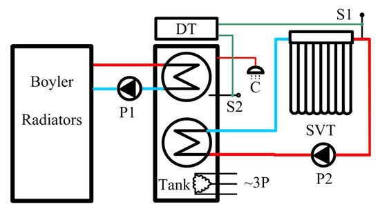
Figure 1.
Heating system diagram.
The report focuses on the summer operating stage. The solar panel consists of a collector and 30 vacuum tubes connected to it, with a total surface area of 2.5 m2. The panel is installed on top of a garage and is not continuously exposed to sunlight, as it is shaded by a neighboring building in the morning. Full sun exposure begins after 10:20 a.m. The distance from the panel to the storage tank is approximately 7 m.
The operation of pump P2 is controlled by a differential thermostat, which receives data from two sensors—S1 located at the collector outlet and S2 positioned in the middle of the storage tank. The thermostat switches on under specific conditions: the temperature in the collector must be higher than 40 °C plus a temperature difference ΔT. This ΔT is the temperature difference between the storage tank and the solar panel, set by the user within the range of 4–20 °C.
If the water temperature in the storage tank is not sufficient for end users, it is heated by electric heaters with a total power of 9 kW supplied from the three-phase network. Measurements were recorded over a 10-day period at the end of August and the beginning of September 2025. The temperature sensors recorded data at regular intervals of one minute (Δt = 1 min) throughout the entire measurement campaign, providing a time-synchronized dataset for both collectors (S1 and S2).
2.2. Artificial Neural Network
The data are based on artificial neural network models whose primary goal is to emulate the functional and structural characteristics of the biological nervous system. This approach is increasingly applied for modeling, simulation, optimization, and prediction of the behavior of various technological objects or processes. An artificial neural network essentially represents a multilayer structure composed of neurons that possess a set of properties adapting to the information-processing workflow.
This flexible architecture offers several advantages, such as the ability to learn and self-organize, the capacity for prediction, and the capability to find optimal solutions for specific tasks. Figure 2 presents a basic structure of an artificial neural network.
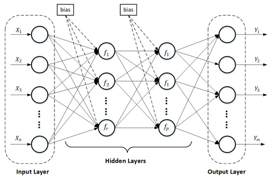
Figure 2.
Schematic diagram of a multilayer artificial neural network.
The tasks that can be solved using artificial neural networks are diverse in nature, most commonly serving as data-archiving structures, simulators, approximators, or classifiers.
The artificial neural network model consists of layers of neurons whose purpose is to transform the input variables into output variables with the highest possible accuracy. Each output from one layer is connected to every neuron in the next layer through weight coefficients. The input/output variables may be represented as binary combinations (from 0 to 1) or as experimental values in either real or normalized form.
The data entering the network are transformed by a discriminant function of the following form:
where is the weight vector representing the connection between the individual layers of the network, is the bias for the neuron, and n is the number of input data points.
In the hidden layers of the artificial neural network, the discriminant function (1) is transformed through a transfer (activation) function.
In this study, the hidden layers use the hyperbolic tangent (tansig) and the logistic sigmoid (logsig) activation functions, respectively, which are standard in MATLAB’s Neural Network Toolbox for nonlinear regression using the Levenberg–Marquardt training algorithm. These functions provide smooth nonlinear mappings and stable gradients, ensuring reliable convergence during training.
The mathematical expressions of these two activation functions, commonly used in artificial neural network models [11], are as follows:
- Sigmoid transfer function:
- Hyperbolic tansig transfer function:
This artificial neural network model forms the basis for developing structures such as multi-layer perceptrons (MLP), adaptive neuro-fuzzy inference systems (ANFIS), self-organizing neural networks (SOM), and others.
When synthesizing a predictive model, it is necessary to introduce criteria for evaluating its performance. The most commonly used accuracy metrics include [12]:
- Mean square error (MSE):
- —experimental input values;
- —values predicted by the artificial neural network (model);
- —number of input values.
- Root mean square error (RMSE):
- Coefficient of determination:
The coefficient of determination is the squared form of the correlation coefficient and explains the dispersion of the predicted values relative to the experimental data.
3. Results and Discussion
To predict the performance of solar collectors or other types of systems using artificial neural network (ANN) methods, a large set of experimental data is required. For the purposes of the present study, the temperatures of the tank, as well as at the inlet and outlet of the solar collector, were measured over a period of 10 days.
Figure 3 shows the temperature curves of the storage tank and the inlet and outlet of the collector. During the ten-day measurement period, a total of 13,622 temperature samples were collected at a fixed sampling interval of one minute, covering the storage tank and both inlet and outlet points of the solar collector.
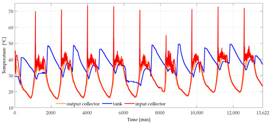
Figure 3.
The temperature curves of the storage tank and the inlet and outlet of the collector.
The collected data were implemented as input training vectors for the artificial neural network model. Figure 4 presents the selected network architecture in the MATLAB R2024b software environment (MathWorks, Natick, MA, USA).
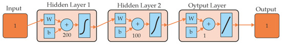
Figure 4.
Artificial neural network topology.
The implemented artificial neural network model consists of one input layer with several neurons corresponding to the length of the input experimental vectors, two hidden layers, and one output layer.
The number of neurons in the hidden layers was determined experimentally to enable training to be performed in a relatively short time while achieving satisfactory accuracy.
During the simulations, it was found that increasing the number of neurons in the hidden layers led to a slowdown in the network’s performance.
The neural network was trained using the Levenberg–Marquardt (trainlm) algorithm. This algorithm offers a relatively high network training speed and is well-suited for solving nonlinear problems.
The activation functions used in the two hidden layers are the hyperbolic tangent (tansig) and the logarithmic sigmoid (logsig) functions, respectively.
Figure 5, Figure 6 and Figure 7 present simulations of the artificial neural network output for the temperature at the tank, as well as the inlet and outlet temperatures of the solar collector, compared to the measured data.
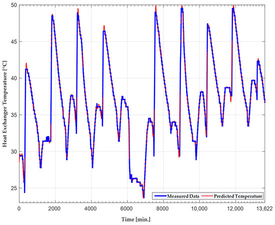
Figure 5.
Predicted and measured values of the storage tank.
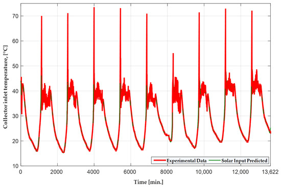
Figure 6.
Predicted and measured values at the collector inlet.
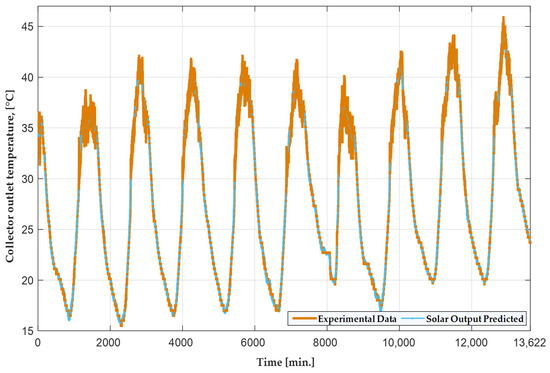
Figure 7.
Predicted and measured values of the collector outlet.
To avoid the risk of overfitting, the input data were divided into three sets (using the divider and function). Seventy percent of the experimental data points were used for training, 15% for validation—so that the network would stop before overfitting occurred—and 15% for independent testing.
In the MATLAB environment, these parameters can be adjusted according to the operator’s (user’s) preference.
As the graphs show, the neural network predicts the discussed variables with relatively high accuracy. The training time is also short, specifically in the order of a few minutes.
To evaluate the model’s performance, Table 1 provides data on the root mean square error (RMSE) and the coefficient of determination (R2) of the network output.

Table 1.
Artificial neural network parameters.
The low RMSE values, together with R2 values close to one, demonstrate the strong predictive capability of the synthesized artificial neural network in this case.
4. Conclusions
This publication presents an approach for modeling artificial neural networks (ANNs) to predict the performance of a solar system with vacuum tubes. The controlled system was analyzed during the summer season over a 10-day period, when the highest amount of solar energy is observed in this geographical region. The authors do not exclude the possibility of extending the study over a longer period to achieve greater reliability of the results.
Based on the collected experimental data, an artificial neural network model was implemented using the Levenberg–Marquardt training algorithm. Through simulations in the MATLAB environment, a suitable network architecture was selected to minimize the mean square error at the output of the ANN model.
The favorable results indicate that the proposed application of artificial neural networks is a promising approach for the development of intelligent automated heating systems for both residential and industrial purposes.
Future research will focus on extending the observation period to the transitional seasons—spring and autumn—to increase the reliability and generalizability of the developed models. Additional efforts will be directed toward comparing different machine learning algorithms, including Random Forest, XGBoost, and deep neural networks, to evaluate their predictive accuracy relative to ANN. Furthermore, the integration of adaptive strategies for intelligent control of hybrid energy systems is planned, which is expected to contribute to higher energy efficiency and sustainability in both residential and industrial applications.
These results also align with the current European Union energy policies, including the European Green Deal, the ‘Fit for 55’ package, the Energy Efficiency Directive (Directive (EU) 2023/1791), and the Renewable Energy Directive (RED III, Directive (EU) 2023/2413). The developed ANN-based approach can therefore be regarded not only as a contribution to intelligent energy management but also as practical support for achieving the EU’s long-term goals of climate neutrality, improved energy efficiency, and accelerated deployment of renewable energy technologies.
Author Contributions
Conceptualization, N.K., M.S. and M.T.; Methodology, N.K. and M.S.; software, M.S.; validation, M.S.; formal analysis, N.K. and M.T.; investigation, N.K.; resources, N.K.; writing—original draft preparation, M.T.; writing—review and editing, M.T.; supervision, M.T.; project administration, M.T. All authors have read and agreed to the published version of the manuscript.
Funding
This research was supported by project “Robotic System with Artificial Intelligence Elements for the Management of Technological Objects and Processes in the Food Industry,” Contract No. 09/25-N, dated 23 July 2025.
Institutional Review Board Statement
Not applicable.
Informed Consent Statement
Not applicable.
Data Availability Statement
The data supporting the findings of this study are available from the authors upon reasonable request.
Conflicts of Interest
The authors declare no conflict of interest.
References
- Fadnes, F.S.; Banihabib, R.; Assadi, M. Artificial neural network model for predicting CO2 heat pump behaviour in domestic hot water and space heating systems. IOP Conf. Ser. Mater. Sci. Eng. 2023, 1294, 012054. [Google Scholar] [CrossRef]
- Rathi, N.K.; Rathi, N. An application of ANN for modeling and optimisation of process parameters of manufacturing process: A review. Int. J. Eng. Appl. Sci. Technol. 2020, 4, 127–134. [Google Scholar] [CrossRef]
- Barteczko-Hibbert, C.; Gillott, M.; Kendall, G. An artificial neural network for predicting domestic hot water characteristics. Int. J. Low-Carbon Technol. 2009, 4, 112–119. [Google Scholar] [CrossRef]
- Bayle, R.; Reyboz, M.; Lomet, A.; Cook, V.; Mermillod, M. Continuously Learning Prediction Models for Smart Domestic Hot Water Management. Energies 2024, 17, 4734. [Google Scholar] [CrossRef]
- Yang, K.T. Artificial Neural Networks (ANNs): A New Paradigm for Thermal Science and Engineering. J. Heat Transf. 2008, 130, 093001. [Google Scholar] [CrossRef]
- Kamble, L.V.; Pangavhane, D.R.; Singh, T.P. Heat Transfer Studies using Artificial Neural Network—A Review. IEJ 2014, 14, 25–42. [Google Scholar]
- Salem, K.M.; Rey-Hernández, J.M.; Elgharib, A.O.; Rey-Martínez, F.J. Optimizing Energy Forecasting Using ANN and RF Models for HVAC and Heating Predictions. Appl. Sci. 2025, 15, 6806. [Google Scholar] [CrossRef]
- Wróbel, J.; Kulawik, A. Calculations of the heat source parameters on the basis of temperature fields with the use of ANN. Neural Comput. Appl. 2019, 31, 7583–7593. [Google Scholar] [CrossRef]
- Balabanova, I.; Georgiev, G. Traffic Load Prediction in Markov Chains using Artificial Intelligence Techniques. In Proceedings of the International Conference on Communications, Information, Electronic and Energy Systems (CIEES), Veliko Tarnovo, Bulgaria, 24–26 November 2022; pp. 1–6. [Google Scholar] [CrossRef]
- Rehman, K.U.; Çolak, A.B.; Shatanawi, W. Artificial Neural Networking (ANN) Model for Convective Heat Transfer in Thermally Magnetized Multiple Flow Regimes with Temperature Stratification Effects. Mathematics 2022, 10, 2394. [Google Scholar] [CrossRef]
- Nasr, M.S.; Moustafa, M.E.; Seif, H.E.; El Kobrosy, G. Application of Artificial Neural Network (ANN) for the prediction of EL-AGAMY waste water treatment plant performance-EGYPT. Alex. Eng. J. 2012, 51, 37–43. [Google Scholar] [CrossRef]
- Ghritlahre, H.K.; Prasad, R.K. Application of ANN technique to predict the performance of solar collector systems—A review. Renew. Sustain. Energy Rev. 2018, 84, 75–88. [Google Scholar] [CrossRef]


Disclaimer/Publisher’s Note: The statements, opinions and data contained in all publications are solely those of the individual author(s) and contributor(s) and not of MDPI and/or the editor(s). MDPI and/or the editor(s) disclaim responsibility for any injury to people or property resulting from any ideas, methods, instructions or products referred to in the content. |
© 2026 by the authors. Licensee MDPI, Basel, Switzerland. This article is an open access article distributed under the terms and conditions of the Creative Commons Attribution (CC BY) license.