Federated Edge Learning for Distributed Weed Detection in Precision Agriculture Using Multimodal Sensor Fusion ^†

Abstract

In this work, our goal is to develop a privacy-preserving distributed weed detection and management system. The proposed work integrates FEL (Federated Learning) and deep learning with multi-modal sensor fusion to enhance the model’s performance while minimising data transfer, latency, and energy consumption. In this study, we used multimodal sensors, such as LiDAR (Light Detection and Ranging), RGB (Red–Green–Blue) cameras, multispectral imaging devices, and soil moisture sensors placed in controlled agricultural plots. Deep learning models, such as Convolutional Neural Networks (CNNs), LSTM–CNN hybrids, and Vision Transformers, were trained using standardized parameters. A proposed Federated CNN (FedCNN) was deployed across multiple edge devices, each locally trained on sensor data without exchanging raw data, using FedAvg and FedProx algorithms. The experimental work revealed that the model FedCNN performed well in comparison to other models and achieved the highest accuracy of 94.1%, precision of 94.3%, recall of 93.9%, F1-score of 94.1%, and AUC of 94.1% during hybrid fusion strategies. We compared the centralized and federated learning performance.

1. Introduction

In the 21st century, agriculture plays an important role. For this research work, environmental monitoring plays a key role. Detection is an important component of precision agriculture because accurate weed identification and treatment have a direct impact on crop yield and resource efficiency. Recent breakthroughs in artificial intelligence (AI) have enabled automatic weed recognition systems; nevertheless, standard centralized machine learning models present substantial obstacles such as high communication overhead, privacy issues, and limited scalability in remote farming contexts. To address these restrictions, federated edge learning (FEL) combined with deep learning and multimodal sensor fusion provides a viable solution by allowing for distributed model training while maintaining data privacy. AI (artificial intelligence) is used to make accurate decisions. Machine learning and deep learning techniques are rapidly being used in agriculture to predict crop diseases, monitor plant health, detect weeds, and classify pests. These applications showcase new and high-impact research fields where deep learning has demonstrated great promise. Simultaneously, sensor technologies are fast improving, allowing for more precise soil fertility assessments and supporting data-driven crop recommendation systems. In this scenario, DL (deep learning) emerged as one of the strongest techniques to solve classification tasks. This technique allows us to handle hidden patterns automatically from raw data. However, the dataset’s characteristics, feature distribution, and task complexity can all affect how well a deep learning model performs on its own. To address the limitations of typical machine learning models, in this paper, we use advanced fusion techniques to combine outputs from different models, improving robustness and accuracy in weed detection. We use a variety of deep learning (DL) architectures, including Convolutional Neural Networks (CNNs), Long Short-Term Memory (LSTM)–CNN hybrid models, and Vision Transformers (ViTs), to capture spatial and temporal patterns in multi-modal agricultural data. Furthermore, as a Federated Convolutional Neural Network (FedCNN) allows for decentralized training among distributed edge nodes, we suggest using one. By keeping raw data locally at each node and sharing only model parameters like weights and biases with the central server, this federated learning (FL) paradigm improves data security and privacy. Additionally, in order to successfully combine multi-modal inputs, including LiDAR, RGB photography, and soil sensor data, three sensor fusion strategies—Early Fusion, Late Fusion, and Hybrid Fusion—are investigated. In practical agricultural settings, this integrated strategy improves energy economy, lowers latency, and protects data privacy while fortifying the system’s predictive performance. Each modality gave complementary information for weed identification: RGB provided texture and colour cues, multispectral devices collected spectral reflectance patterns, LiDAR delivered structural depth information, and soil sensors supported contextual environmental conditions. For robustness, the following three sensor fusion techniques were used: Early Fusion (feature-level concatenation), Mid Fusion (intermediate feature aggregation), and Late Fusion (decision-level integration).

This study contains five sections, where Section 1 provides the information and background details of weed detection, and Section 2 presents related work of weed detection using deep learning, along with federated learning. Section 3 discusses the entire roadmap of the proposed model for distributed weed detection in precision agriculture using multimodal sensor fusion. Section 4 presents the results and discussion, followed by the conclusion and future scope.

2. Related Work

The authors Xia et al. [1] used a multi-modal data-fusion-technique-based framework for weed resistance assessment. The authors demonstrated how combining various sensor modalities may efficiently capture geographical variability and create a strong link between multi-modal features and resistant weed concentrations. The experimental work revealed that late fusion gave the best result of R² of 0.777 and RMSE of 0.547. Salve, P., et al. [2] used several classification tasks to identify plant types. The authors used multi-modal fusion techniques to enhance the accuracy of plant type detection. Multiple feature types, such as leaf spectral signatures, leaf colour, and morphological form features, were used to process plant image datasets. The Genetic Algorithm-based Regression (GAR) model achieved an accuracy of 98.03%. Behera, S., et al. [3] presented that how FL helps to detect the crop. The author conducted the experimental work where DL models were considered to predict the crop disease.

Li, L., et al. [4] developed a framework that allows for smart farming. The authors’ objective was to design a lightweight FL framework, which is called VLLFL. The mentioned framework allows for identifying crop health and maintaining pesticides. To optimize crops, the authors used FL along with deep learning models. Their experimental observation found that VLLFL obtained a 14.53% improvement and reduced communication rounds by 99.3%. Anagnostopoulos, C., et al. [5] discussed how FL is helpful in an AIoT environment. The authors discussed challenges and present problems, etc. The authors’ objective was to develop a novel classification strategy. The classification approach name is MMFL, which is used in the four application areas. Hussaini, M., et al. [6] developed a deep learning model for crop detection. The authors explored how FL is used for crop identification, as well as weed detection. The DL model YOLOv8 was used to train the dataset and apply the FL model FedAvg. The model was trained in homogeneous and heterogeneous environments. The CornWeed dataset was employed, which consists of 3575 annotated images. The experimental observation revealed that YOLOv8 performs well in comparison to the other two versions of the YOLO algorithm in terms of the performance metrics of accuracy, memory space, and CC (computational cost) when training is considered. Mamba Kabala, D., et al. [7] developed a model that helps with crop disease. The authors used FL models to protect the data. The PlantVillage dataset was taken and used to develop deep learning models, such as ViT, using FL. Rehman, M. U., et al. [8] developed a model that allows for conducting weed detection using an advanced deep learning algorithm. The authors considered the family of YOLO algorithms to detect weed identification. Their model achieved a precision of 72.5% and a recall of 68.0%.

3. Proposed Model for Federated Edge Learning for Distributed Weed Detection

Data Division: In this section, we split the dataset into three parts, and these include training at 70% and testing at 15%, with the remaining 15% used for validation purposes. Model Architectures and Parameters: Here, there are different deep learning models employed for weed detection, and these are mentioned as follows:

CNN (Convolutional Neural Network): We used a CNN with five layers, and each layer had a kernel size of 3 × 3, ReLU activation, and batch normalization. The next model is LSTM–CNN: This is a hybrid model which combines an LSTM layer with 128 units to capture patterns. Vision Transformers (ViTs) are used with 12 attention heads and patch sizes of 16 × 16, along with feedforward networks of 2048 units. Hyperparameters are used for different models, and these are: LR: 0.01, batchsize: 32 for local training and 64 during the centralized evaluation. Apart from this, we also used the Adam optimizer, where β1 = 0.9 and β2 = 0.999. The dropout we considered was 0.5 to avoid overfitting. The binary cross-entropy loss was considered for weed classification.

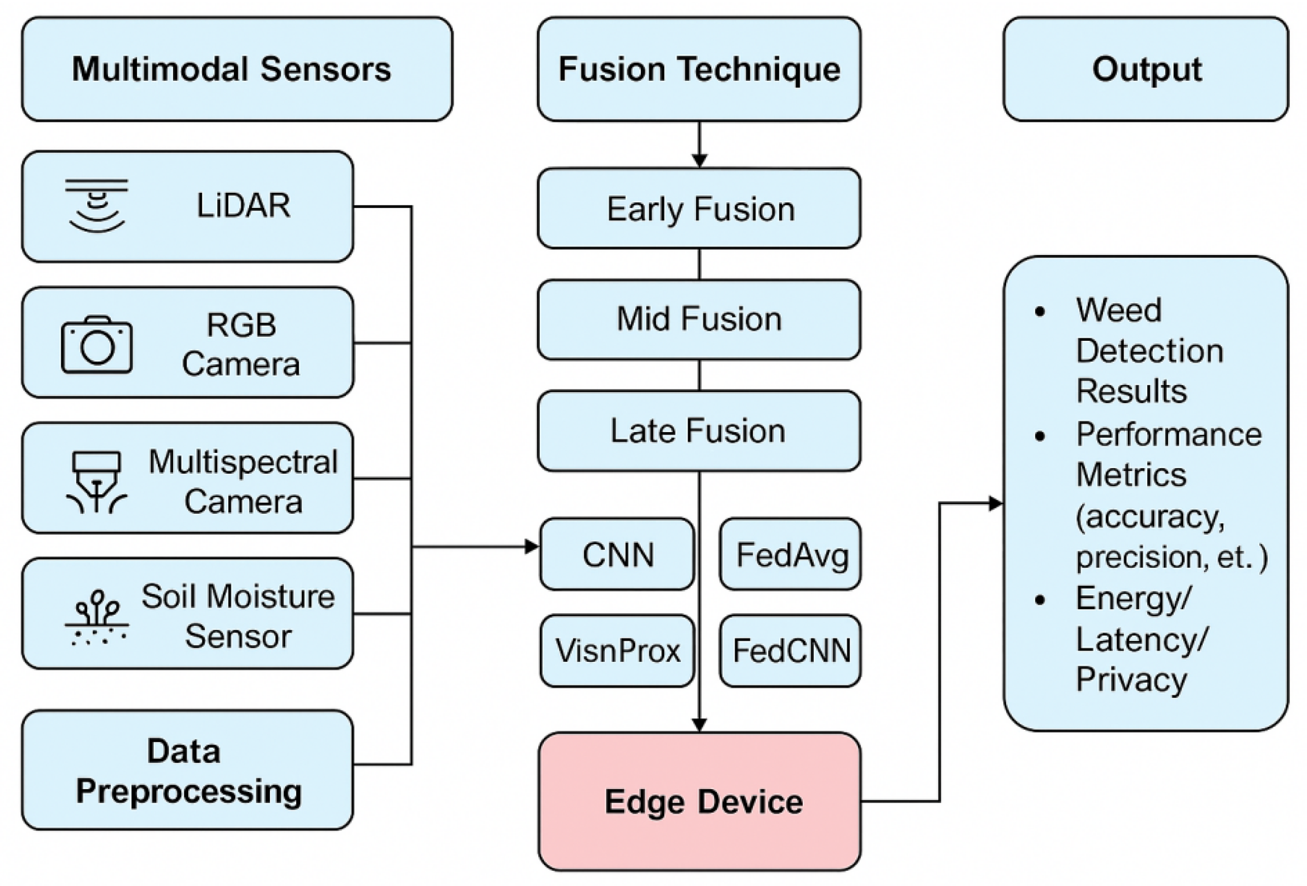
The above-mentioned Figure 1 presents the privacy preservation weed detection system, which consists of seven phases. These phases are described as follows: Phase 1: In this phase, we used multi-modal sensors to collect data from several sources. In order to obtain the plant structure, we used a LiDAR sensor that captures 3D spatial types of data. For high-resolution images, an RGB camera is used to take a snapshot of the weeds. Similarly, a soil moisture sensor was used for collecting real-time moisture levels. Our objective was to collect the data from multi-modal sensors to monitor weed growth patterns. In this research paper, we used a publicly available dataset named “PlantVillage”. We refer the dataset from this [https://www.kaggle.com/datasets/emmarex/plantdisease (accessed on 21 May 2025)] source and the repository name is Kaggale. Apart from this dataset, we also collected data of in-field images using different sensors (including smartphone-based cameras). So, we employed a hybrid dataset for identifying weeds. Phase 2: During the preprocessing stage, we removed noise and performed normalization techniques. To enhance the image quality, RGB/multispectral images were used. Before model selection, we performed extensive data preparation and analysis. The outcome of this phase was cleaned data, which was processed at the edge level to extract a lightweight CNN-based model. To minimize computational load, we used leaf shape, colour histogram, spectral signatures, and soil metadata that were recovered using lightweight CNN-based models after prepossessing. This procedure minimized communication overhead and protected privacy by ensuring that only pertinent, condensed features were kept. Phase 3: Feature Extraction and Multimodal Sensor Fusion. In this phase, we identified the relevant features which were extracted from the weed images. These features are called multi-modal features. These features were further utilized for data fusion purposes. The collected sensor data were further fused into the following three categories: Early Fusion: In this case, our collected sensors’ raw data was converted into a unified format. Mid Fusion: The sensor’s data was preprocessed independently and the intermediate features were fused. Late Fusion: This was used to combine the final sensor data and provide the average output. This technique was used to classify the weeds and estimate the performance metrics. Phase 4: In this phase, we used deep learning models that properly classified the weeds. The fused data was passed into the deep learning model to deep dive, process, and detect the identified weeds. For extracting the spatial features, we used DL models; the LSTM–CNN model was used for spatial–temporal analysis purposes. It is also called a hybrid model. Similarly, a vision transformer (ViT) was used for the analysis of high-dimensional data.

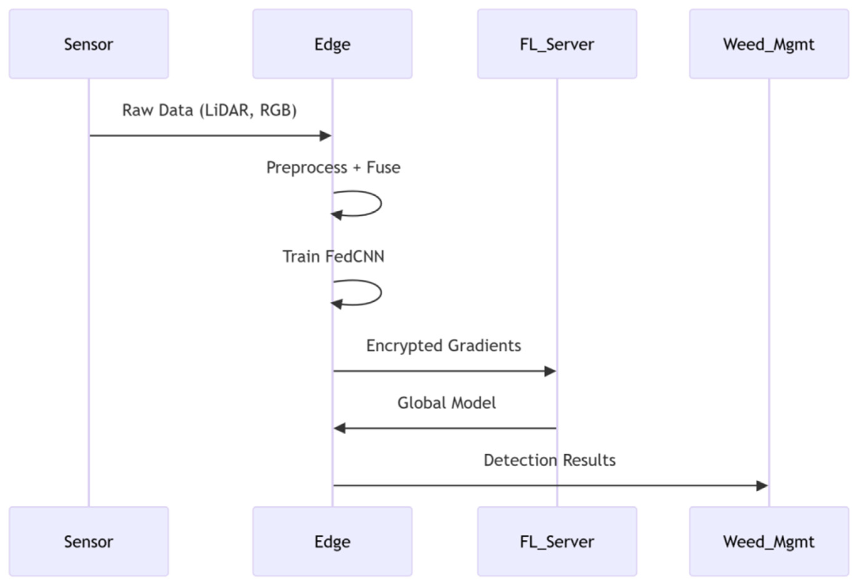
The above Figure 2 represents the sequence diagram for Federated Weed Detection, which discusses the time-ordered interactions between the different associated components. Here, the components include FL server, weed management, sensors, and edge, etc. Data is usually collected from the different sensors and passed into the edge device. The sequence diagram discusses how the components interact with each other, and it follows hybrid fusion and local FedCNN training. Then, the model is encrypted and sent to a federated learning server. In the FL server, the FedProx algorithm is used for aggregation. The FL server sends the updated global model to the edge devices. At the end, the edge device is responsible for deploying the model for real-time weed classification. In this paper, the weed detection accuracy obtained is about 94.1%.

4. Results and Discussion

Deep learning model creation and processing:

The acquired RGB and LiDAR datasets, as well as other sensor data, were preprocessed through a series of procedures to ensure data quality and compatibility for deep learning models. Images and point cloud data were first aligned using GPS coordinates, then noise and outliers were removed. The data was scaled to 224 × 224 pixels for deep learning models and normalized with min–max scaling to improve convergence during training. Data augmentation techniques such as rotation, flipping, and brightness modifications were used to boost dataset diversity while reducing overfitting. Validation was performed using a stratified 80/20 train–test split combined with 5-fold cross-validation to ensure model generalization. Model performance was assessed using accuracy, precision, recall, F1-score, AUC, latency, and energy consumption, enabling a holistic evaluation of both predictive quality and computational efficiency. DL models, including CNNs, LSTM-CNN hybrids, and Vision Transformers, were used. A FedCNN model was distributed across many edge nodes, allowing for decentralized training without exchanging raw data. For model performance measures, we used different metrics like accuracy, precision, recall, F1-score, AUC, latency, and energy. The FEL (Edge) accuracy was 94.1%, the Latency was 120 ms, the energy consumption was 300 (mWh), and the privacy risk level was low. Conclusion: The combination of FEL and multi-modal sensor fusion provides a reliable and scalable approach for weed detection in precision agriculture. By processing data locally and collaboratively at the edge, the system achieves high accuracy, decreases response time, lowers energy consumption, and preserves data privacy.

Table 1. Performance comparison of different fusion strategies with FedCNN.

Fusion Strategy	Accuracy (%)	Precision (%)	Recall (%)	F1-Score (%)	AUC (%)
Early Fusion	92.8	92.9	92.5	92.7	92.8
Mid Fusion	93.5	93.6	93.2	93.4	93.5
Late Fusion	93.7	93.9	93.4	93.6	93.7
Hybrid Fusion	94.1	94.3	93.9	94.1	94.1

discusses the performance metrics of the different feature fusion techniques. There are multiple fusion techniques implemented, and these are Early Fusion, Mid Fusion, Late Fusion, and Hybrid Fusion. All these fusion techniques are used against the FedCNN model, which is used to perform weed identification. It is observed that the Hybrid Fusion technique obtained the highest accuracy of 94.1%, precision of 94.3%, recall of 93.9%, F1-score of 94.1%, and AUC-ROC of 94%. It also observed that Early Fusion obtained 92.8% accuracy.

The above-mentioned

Table 2. Comparison of deep learning models for weed detection.

Model	Architecture Type	Accuracy (%)	Precision (%)	Recall (%)	F1-Score (%)	AUC (%)
CNN	Convolutional Neural Net	90.5	91	89.9	90.4	90.6
LSTM-CNN Hybrid	Spatial + Temporal Fusion	92.3	92.5	91.8	92.1	92.4
Vision Transformer	Attention-based Transformer	93.5	93.2	93.1	93.1	93.4
FedCNN (Proposed)	Federated CNN (Edge Device)	94.1	94.3	93.9	94.1	94.1

discusses the comparison of different deep learning models for weed identification. It is observed that the best model is FedCNN, and its accuracy is 94.1% in comparison to the other models. The AUC-ROC curve obtained 94.1%, with an F1-score of 94.1%. FL uses distributed edge devices for training instead of centralizing data, which improves generalization while keeping privacy. The traditional model, the CNN, obtained the lowest accuracy of 90.5%. CNNs cannot capture complex spatial patterns as well as hybrid or transformer-based architectures.

Table 3. Centralized vs. federated edge learning (FEL) performance.

Learning Approach	Accuracy (%)	Latency (ms)	Energy Consumption (mWh)	Privacy Risk Level
Centralized Learning	94.5	250	510	High
Federated Edge Learning (FEL)	94.1	120	300	Low

presents a comparison between centralized and federated edge learning. It is observed that the centralized model performs a little bit better than the federated learning model. FEL reduced the latency by 120 ms as well, and energy consumption dropped from 500 mWh to 300 mWh. It helps to protect privacy more in comparison to the centralized model.

The above

Table 4. Comparison of FL algorithms (FedAvg vs. FedProx).

FL Algorithm	Accuracy (%)	Precision (%)	Recall (%)	F1-Score (%)	AUC (%)	Latency (ms)	Energy (mWh)
FedAvg	93.7	93.6	93.5	93.5	93.6	150	350
FedProx	94.1	94.3	93.9	94.1	94.1	120	300

presents the comparison between FL algorithms. We compare the two FL algorithms, FedAvg and Fed Prox. It is observed that the FedProx Fl algorithm’s accuracy is 94.1%, with a precision of 94.3% and F1-score of 94.1%. The algorithm FedAvg is still competitive, but its performance is slightly lower because it is sensitive to non-IID (not independent and identically distributed) data, which makes convergence less stable.

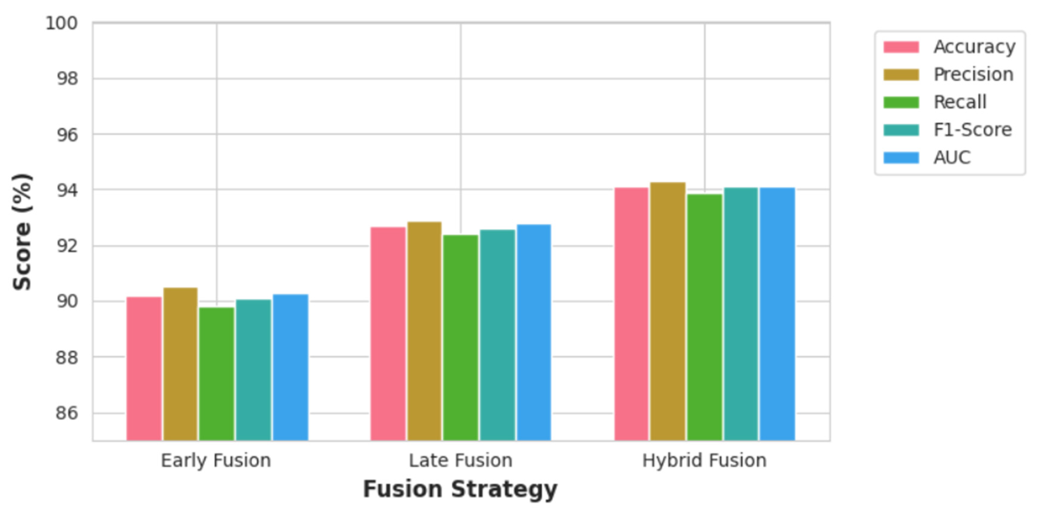
In Figure 3, we compare the three different fusion techniques for FL weed detection using the five performance metrics. The Hybrid Fusion technique performs well, achieving an accuracy of 94.1% accuracy and precision of 94.3%. Additionally we also observed that Late Fusion (+1.4%) and Early Fusion (+3.9%) yield satisfactory results. These findings help us understand that Hybrid Fusion’s performance is good at balancing between precision and privacy preservation, but Late Fusion may be preferable for resource-constrained edge deployments.

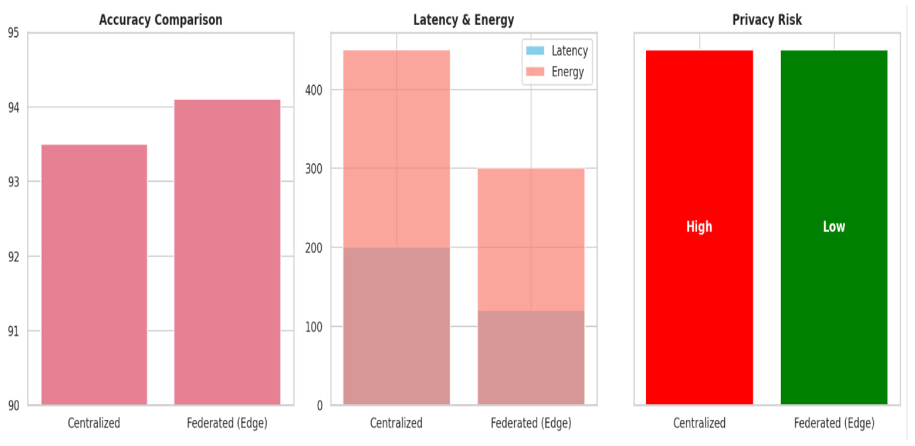
In Figure 4, we estimate the critical trade-offs between the centralized and federated learning environment, where our objective is weed detection. The FedCNN obtained the highest accuracy (94.1% vs. 93.5%). The AUC-ROC curve is most important to measure the cost of misclassifying (both TPR and TNR) for weed detection. When the dataset is imbalanced, traditional metrics like accuracy may not be ideal. In contrast, the ROC curve helps to visualize the trade-off between TPR and TNR. The AUC gives a solid measure of the model’s ability to tell the difference between things by translating this performance into a single number.

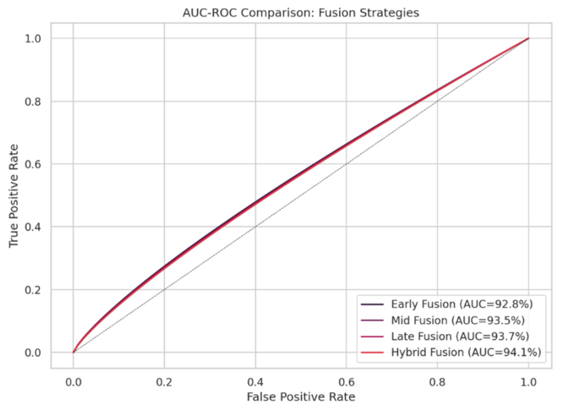
Figure 5 presents the AUC-ROC curve for fusion strategies that are used to determine the contribution to the classification accuracy. During our experimental observation, we found that our Hybrid Fusion approach obtained the highest AUC of 94.1%. This demonstrates how early weed detection is possible. The other two fusion techniques were also utilized and obtained performances with AUCs of around 93.7% and 93.5%.

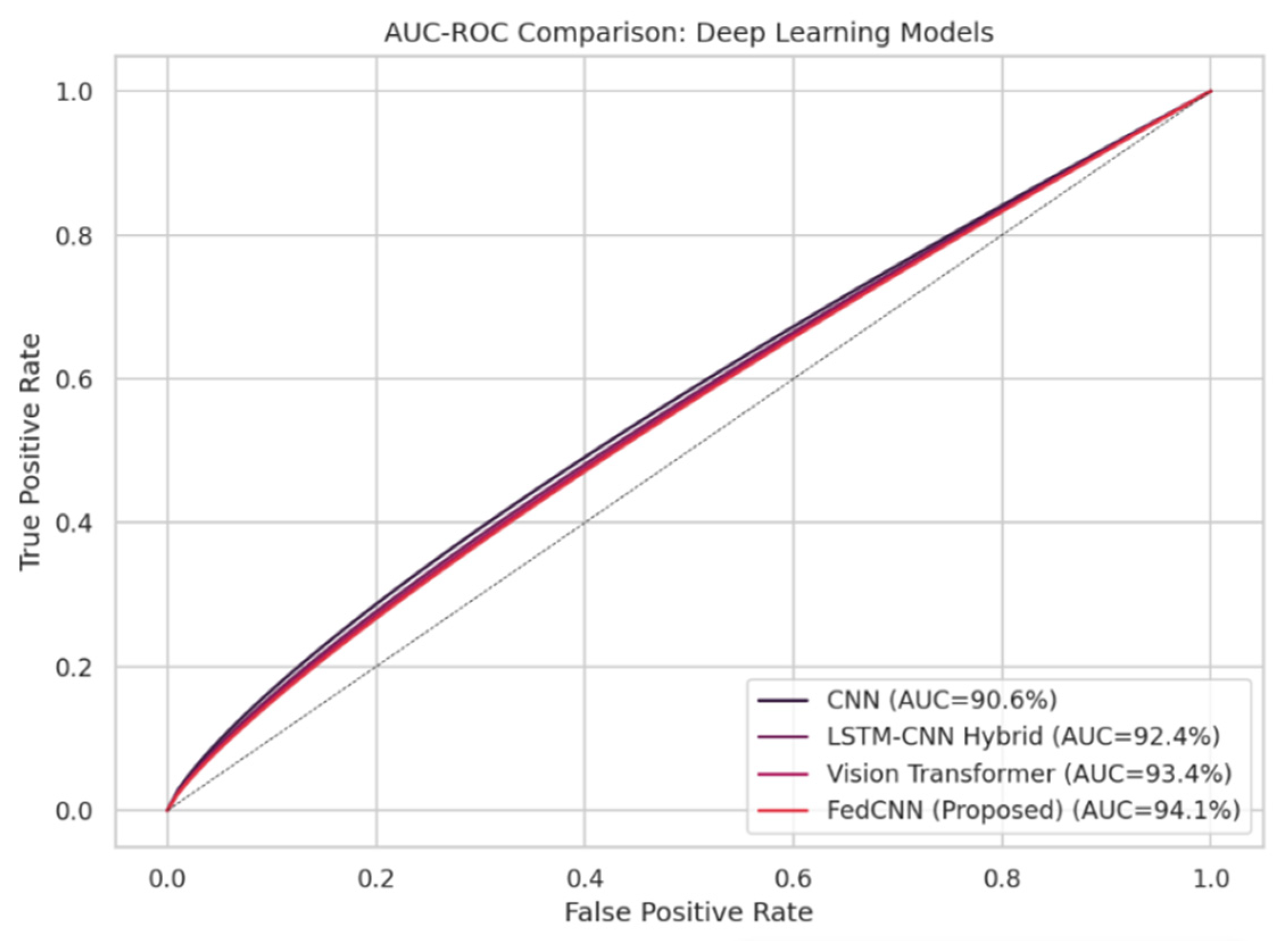
Figure 6 presents the AUC-ROC curve, which is used to detect weeds using deep learning models. It is observed that FedCNN obtained the highest AUC score of 94.1% as compared to the other DL models. Similarly, CNN obtained an AUC score of 90.6%, while Vision Transformer’s AUC score is 93.4%. In this graph, the top left is the better model. The FedCNN AUC is one of the general models with a low TFR. It is clear from these results that federated learning and hybrid designs can help models work better on devices that are spread out. This metric is suitable for handling binary class classification. If the AUC is greater, it means that the model or fusion strategy can make more accurate predictions when the decision boundaries change. This is very important in edge-device federated learning settings like FedCNN, where the conditions for a threshold may change on the fly based on how the data is distributed and how it is deployed.

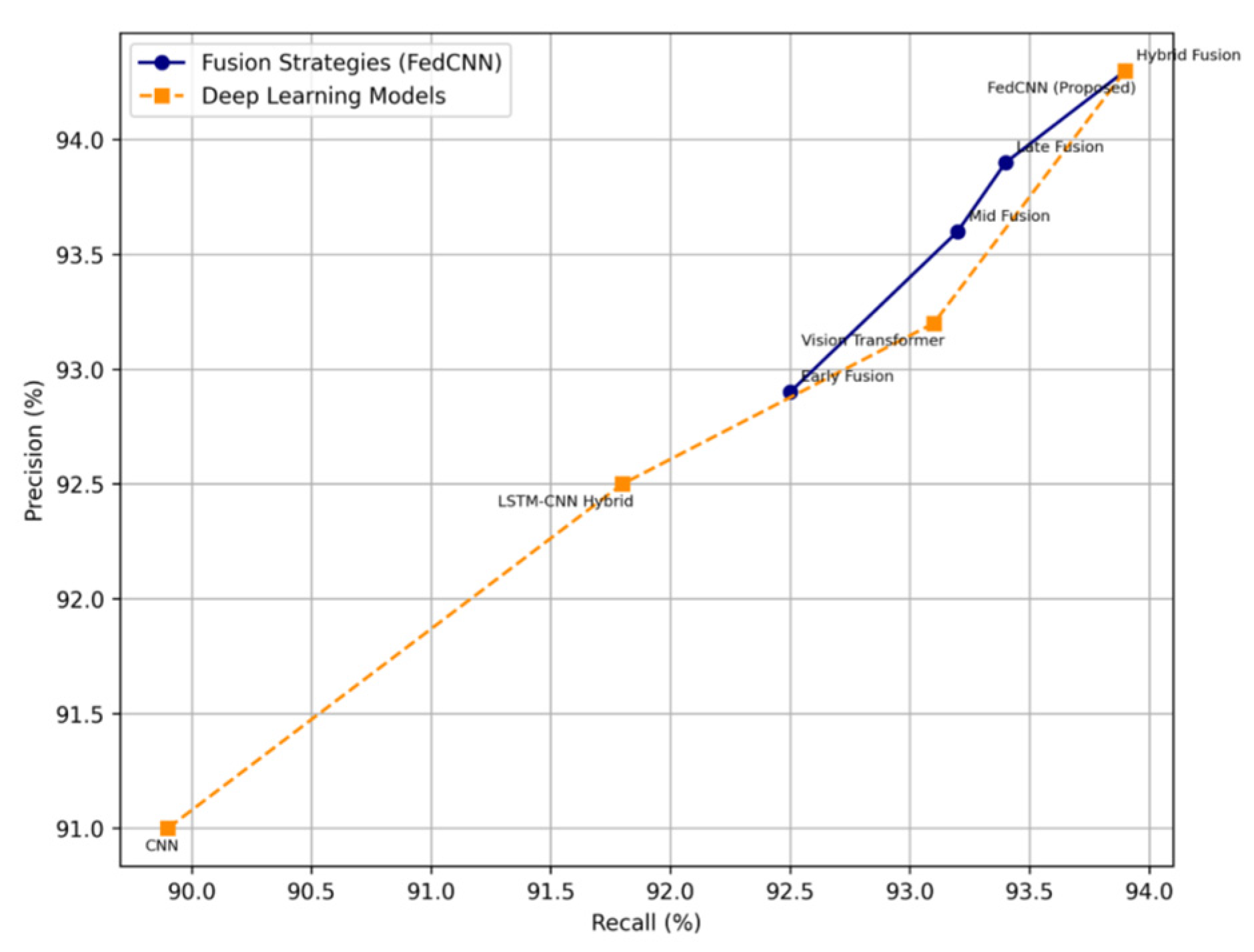
In the above-mentioned Figure 7, we plot the precision and recall curve for weed classification using the precision and recall scores of the different models. We evaluate the different machine learning models that are used for a real-time insect detection and monitoring system. We use the PR curve, especially when the dataset is imbalanced. This allows researchers to visually assess how well each method balances precision and recall, which helps them choose the highest-performing and most reliable approach for deployment.

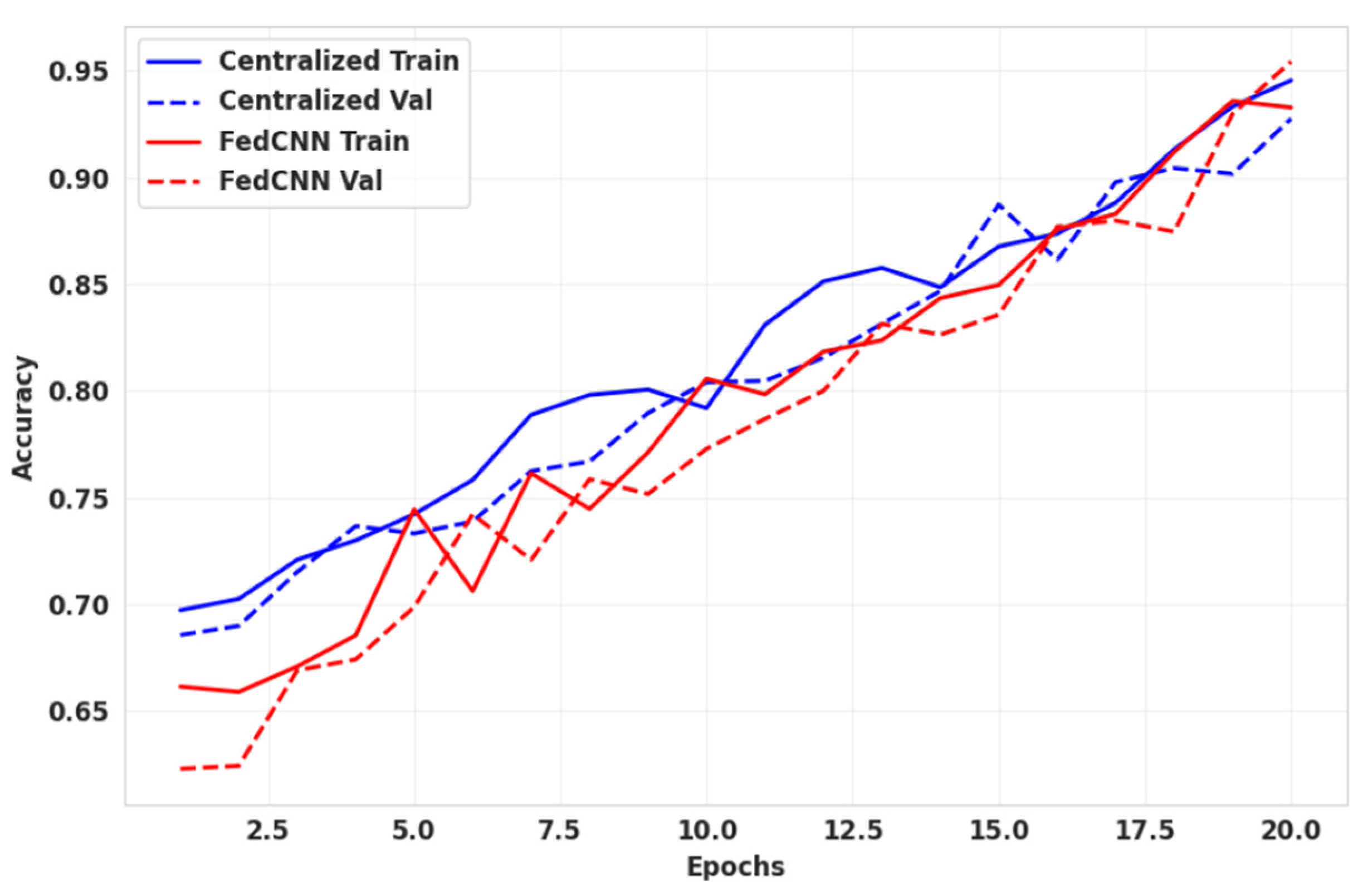
In Figure 8, we compare the prediction accuracy of the federated learning CNN model and the centralized model concerning the number of epochs. The solid line indicates how the model behaves on the training data, and the dashed line visualizes validation accuracy. This visualization describes how the model behaves the unseen data, whether it is a generalized model or not. The red line shows the highest validation accuracy as compared to the centralized training accuracy. The FL model exhibits slightly slower convergence because of decentralized updates.

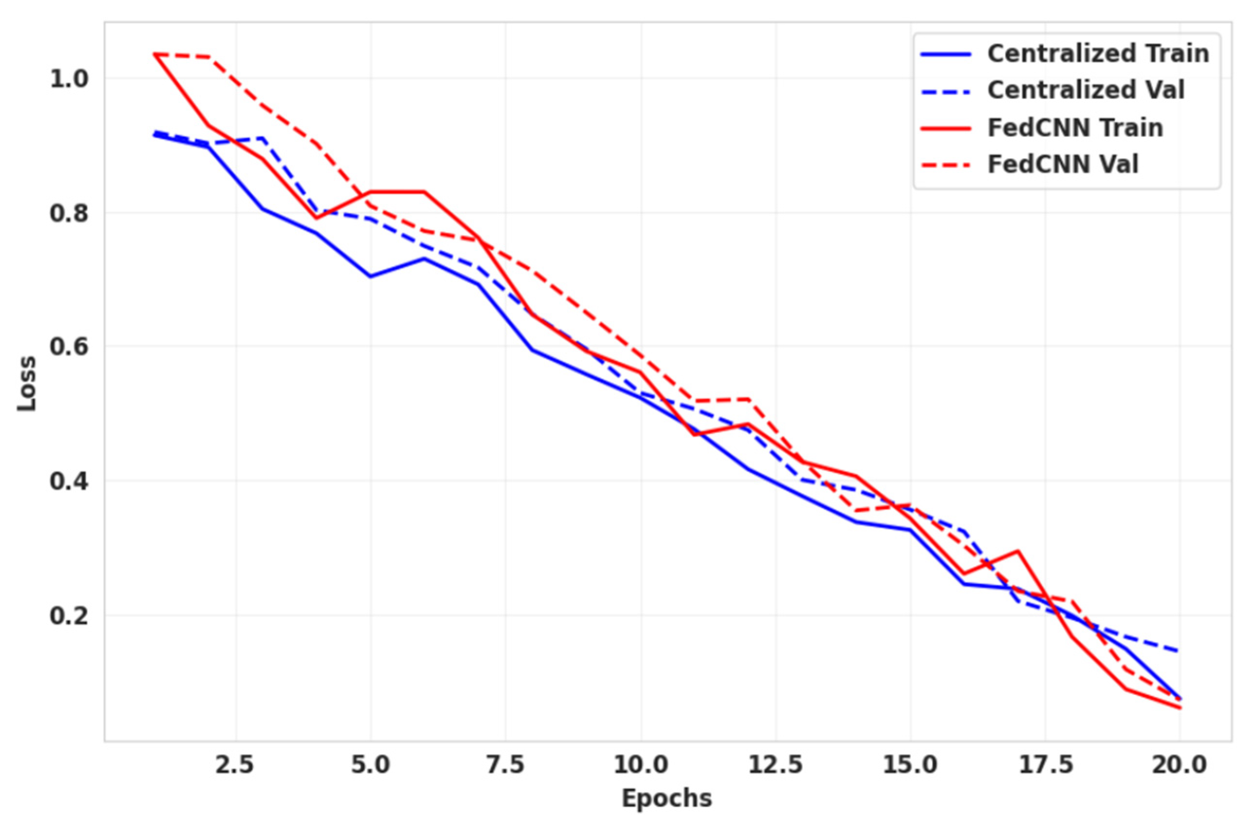
The above-mentioned Figure 9 discusses the relationship between training and validation losses. During training, it estimates the cross-entropy loss. If the loss is less than identified, it is better optimized. The red line, denoting loss, is the lowest one, which is compared to the centralized loss represented as a blue line.

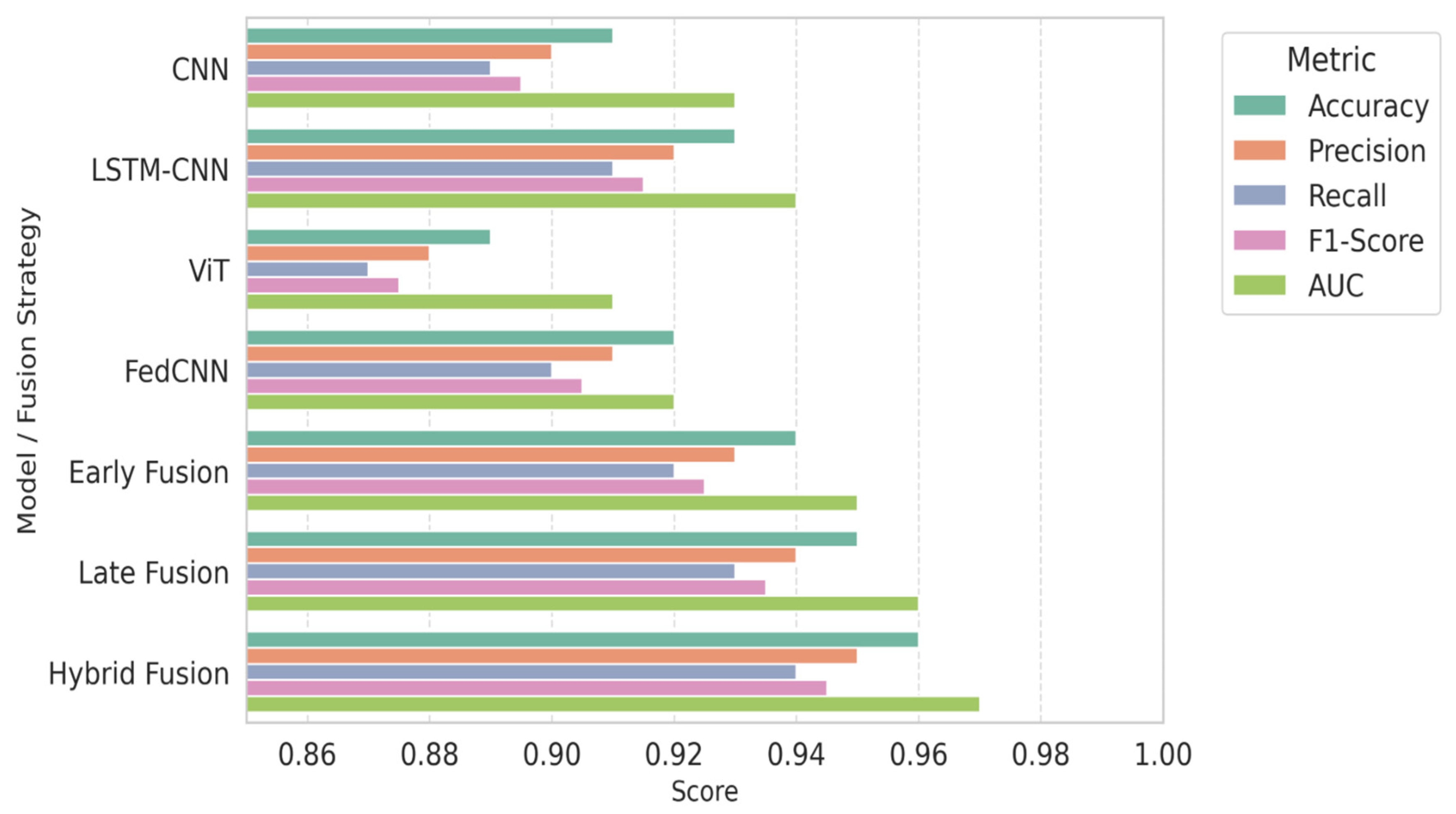
Figure 10 demonstrates the performance of different deep learning models and distributed FedCNN. This graph compares the performance of several deep learning models—CNN, LSTM–CNN hybrid, Vision Transformer (ViT), and the distributed FedCNN—across the following three fusion strategies: Early Fusion, Late Fusion, and Hybrid Fusion. The above figure depicts that the Hybrid Fusion model performs well in comparison to the other models. The model FedCNN shows the best result, especially FedCNN. Apart from this, Vision Transformer also performs well, with strong generalization capabilities.

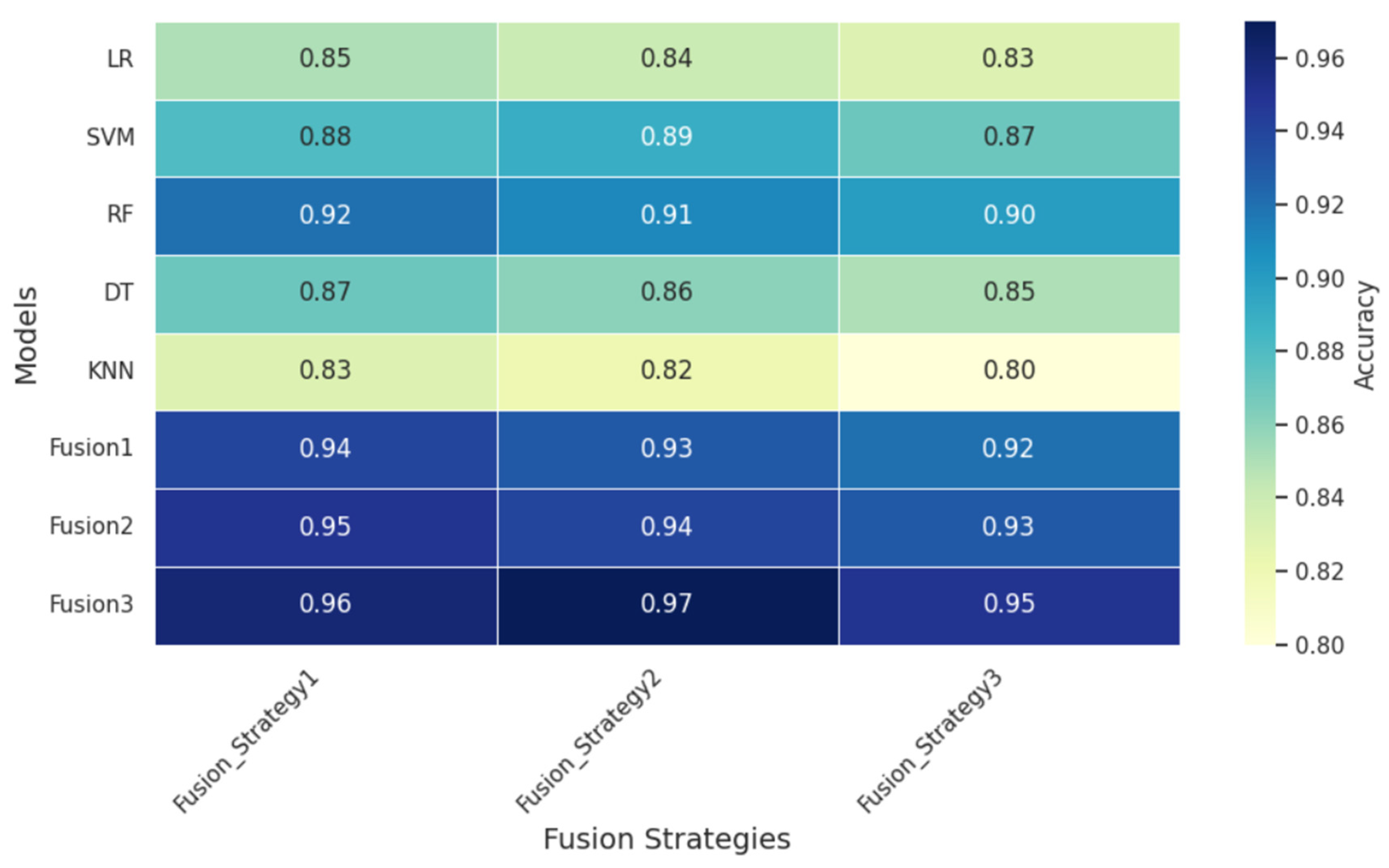
The above-mentioned Figure 11 presents a heatmap representation of the individual machine learning models and fusion strategies. We compare the fusion strategies side by side.

5. Conclusions

This paper discussed a combined approach for weed detection in precision agriculture. We used fusion techniques along with federated edge learning to detect weeds from the PlantVillage datasets. From our experimental observation, it is observed that the Hybrid Fusion technique provides good results. The performance achieved 94.1% accuracy because of the three combined fusion strategies. The proposed Federated CNN (FedCNN) achieved 94.1% accuracy, a recall of 94.3%, and an F1-score of 94.1%. Overall, the proposed FedCNN with Hybrid Fusion and FedProx optimization provides a robust, efficient, and privacy-preserving method for weed detection, allowing real-time, sustainable, and scalable smart farming applications.