Proceeding Paper

Model-Free Control for Greenhouse Automation with Hardware-in-the-Loop and Raspberry Pi Implementation †

1
Departamento de Automatización y Control Industrial, Escuela Politécnica Nacional, Quito 170525, Ecuador
2
Colegio de Ciencias e Ingenierías, Universidad San Francisco de Quito (USFQ), Quito 170157, Ecuador
*
Author to whom correspondence should be addressed.
Presented at the XXXIII Conference on Electrical and Electronic Engineering, Quito, Ecuador, 11–14 November 2025.
Eng. Proc. 2025, 115(1), 15; https://doi.org/10.3390/engproc2025115015
Published: 15 November 2025
(This article belongs to the Proceedings of The XXXIII Conference on Electrical and Electronic Engineering)

Abstract

This paper presents the design, implementation, and experimental validation of a model-free control strategy for greenhouse climate automation. The proposed approach integrates a real-time embedded controller based on a Raspberry Pi within a Cyber-Physical System (CPS) framework. A Hardware-in-the-Loop (HIL) simulation architecture was developed, where the physical controller interacts with a high-fidelity digital twin (DT) of the greenhouse modeled in MATLAB/Simulink. This configuration allows a realistic assessment of the control performance, enabling the evaluation of system dynamics, actuator limitations, and response to disturbances before actual deployment. The control strategy is based on an intelligent Proportional–Integral (iPI) model-free algorithm, which avoids reliance on explicit process modeling and is well-suited for nonlinear and time-varying environments. Experimental results demonstrate the effectiveness, robustness, and practical feasibility of the proposed approach for real-time greenhouse automation. The use of low-cost hardware and the modular nature of the system make it scalable and attractive for precision agriculture and educational applications.

1. Introduction

Climate control in greenhouses is inherently complex due to the system’s nonlinear, multivariable nature and unpredictable meteorological disturbances [1]. Maintaining optimal internal conditions like temperature and humidity is crucial for crop yield, energy efficiency, and sustainability. Traditional control strategies rely on mathematical modeling, such as energy and thermal balance models [2,3,4] or black-box identification techniques [1,5]. However, their implementation is challenged by nonlinear dynamics, parameter variability, and weather uncertainty. As a result, PID and Boolean logic controllers remain common, despite tuning difficulties and poor performance under varying conditions.
MFC has emerged as a viable alternative that avoids explicit plant modeling [6]. Based on ultra-local models and intelligent PI/PID (iPI/iPID) controllers, MFC offers ease of tuning, robustness, and strong tracking performance, as demonstrated in several domains [7,8]. In agriculture, the growing need for adaptive and energy-efficient control systems highlights the limitations of conventional automation in dynamic environments [9].
Recent advances like CPS offer a promising approach by integrating physical processes with real-time computation and control. However, agricultural CPS implementations mostly remain in simulation, with limited deployment. Similarly, hybrid control strategies—combining continuous and discrete actions—are still underutilized in smart farming [10,11]. IoT-based greenhouse solutions, such as that in [12], have automated basic monitoring using Raspberry Pi and sensors, yet typically rely on rule-based control lacking adaptability to greenhouse dynamics.
This study presents the design and experimental validation of a hybrid model-free control strategy for greenhouse climate regulation within a CPS framework. The system integrates a Raspberry Pi as an embedded controller and a high-fidelity digital twin in MATLAB/Simulink R2025b under an HIL architecture. This setup enables realistic testing and tuning and demonstrates the feasibility of deploying MFC in real-time environments. Key contributions include the use of low-cost embedded hardware, data-driven control, and HIL-based validation for future smart agriculture applications.
The remainder of this paper is organized as follows. Section 2 introduces the DT of the greenhouse. Section 3 describes the intelligent PI control strategy. Section 4 presents the implementation of the controller on the Raspberry Pi. Section 5 discusses the experimental results obtained through the HIL setup. Finally, Section 6 summarizes the main findings and outlines future research directions.

2. Digital Twin for a Greenhouse Climate System

This section introduces the digital twin representation of the greenhouse climate system, structured in two parts. The first part formulates the dynamic behavior of the microclimate through mass and energy balance differential equations, which define the physical model of the system [2,11,13,14]. The second part establishes the operating point around which the nonlinear control is designed, providing the corresponding steady-state values used for linearization and control synthesis.

2.1. Differential Equations That Describe the Greenhouse Dynamics

Figure 1 shows the inputs, outputs, and disturbances acting on the greenhouse system, while in Equations (1) and (2) the differential equations that govern the dynamic of the greenhouse microclimate, obtained from [2]:
d T i n d t = 1 ρ · C p · V · Q h + S i γ · Q f o g   ( T i n T o u t ) · V t V + U · A ρ · C p · V ,
d W i n d t = 1 ρ · V · Q f o g + E V t W i n W o u t .
where T i n is the indoor air temperature (°C), T o u t is the outdoor temperature (°C), ρ is the air density (kg· m 3 ), C p is the specific heat of air (J· kg 1 · K 1 ), V is the greenhouse volume ( m 3 ), Q h is the heat provided by the greenhouse heater (W) which is not used for this project (then Q h = 0 W), S i is the intercepted solar radiant energy (W), γ is the latent heat of vaporization (J· g 1 ), Q f o g is the water capacity of the fog system (water vapor mass per second, in (g· s 1 )), V t is the ventilation rate ( m 3 · s 1 ), U is the overall heat transfer coefficient (W· m 2 · K 1 ), A is the greenhouse of surface area ( m 2 ), W i n and W o u t are the interior and exterior humidity ratios (water vapor mass of dry air, in (g· m 3 )), respectively, and E is the evapotranspiration rate of the plants (g· s 1 ), which is expressed by Equation (3) below:
E = α S i γ β T · W i n .
where α is the coefficient to account for shading and leaf area index ( α = 0.125), and β T is the coefficient to account for thermodynamic constants and other factors affecting evapotranspiration (in this specific case, β T = 0).
The intercepted radiant solar energy results from solar radiation outside the greenhouse that strikes the roof area; therefore, its mathematical expression is shown in Equation (4) below.
S i = S r · A .
where S i is the intercepted radiant solar energy (W), S r is the solar radiation external to the greenhouse (W· m 2 ), and A is the greenhouse of surface area ( m 2 ).

2.2. Steady State Values Around Operation Point

If constant environmental conditions are considered, Equations (1) and (2) are assumed to be zero, and the system can be analyzed at the operating point (as in [11,14]). Following the approach in [11], the values of the constants and input variables for the greenhouse under study were used to determine the operating point.
Applying these values, the operating points for temperature ( T i n ) and absolute humidity ( W i n ) inside the greenhouse are calculated using Equations (5) and (6).
T i n 0 = 1 ρ · C p · V t ¯ + U · A · A · S r ¯ γ · Q f o g ¯ + T o u t .
W i n 0 = 1 V t ¯ + β T · Q f o g ¯ + α · A · S r ¯ γ + V t ¯ · W o u t ¯ .
The result of the calculation is obtained T i n 0 = 31.997 and W i n 0 = 7.460, which are the operating points around the nonlinear system that will work.

3. Intelligent PI Controller Approach

One promising feature of this approach is the use of an ultra-local model, which replaces the need for a precise process model and includes a real-time estimator that dynamically updates the system behavior [6]. Although the iPID framework allows different configurations (iP, iPI, iPID), in this work, we adopt the iPI structure, which is sufficient for the class of processes considered. The design and implementation details of the iPI controller are presented below.
The ultra-local model for an SISO system is represented as follows:
y ˙ ( t ) = F ( t ) + α u ( t ) .
where F ( t ) captures the unmodeled dynamics and disturbances, α R is a positive design parameter chosen to align the magnitudes of y ˙ ( t ) and α u ( t ) , and u ( t ) is the control input.
The control objective is defined through the tracking error:
e ( t ) = R ( t ) y ( t ) .
Here, R ( t ) denotes the desired reference, while y ( t ) corresponds to the system output. This error metric provides the foundation for designing the control law, ensuring that the system output converges to the reference value with minimal deviation, even in the presence of disturbances or model uncertainties.
Considering that an iPI controller is enough for the proposal objectives, the control law takes the following form:
u ( t ) = 1 α F ( t ) + R ˙ ( t ) + K P e ( t ) + K I 0 t e ( τ ) d τ .
where K p and K i are the proportional and integral gains, respectively, and are tuned to ensure accurate tracking of R ( t ) . Substituting the model equation into the control law results in the closed-loop error dynamics:
e ˙ ( t ) + K P e ( t ) + K I 0 t e ( τ ) d τ = 0 .
This suggests that disturbances and unmodeled components within F ( t ) are effectively canceled. To estimate y ˙ ( t ) , various methods can be employed, such as numerical differentiation or filtering. A first-order low-pass filter is commonly used, defined as
H L P ( s ) = K L P s T L P s + 1 .
where K L P and T L P are the gain of the filter and the time constant, chosen to balance the noise reduction and delay. Using this filter, the disturbance estimation is given by the following:
F ^ ( t ) = y ˙ ( t ) α u ( t ) .
where y ˙ ( t ) represents the estimated derivative of the output of the system.

3.1. iPI Controller Scheme

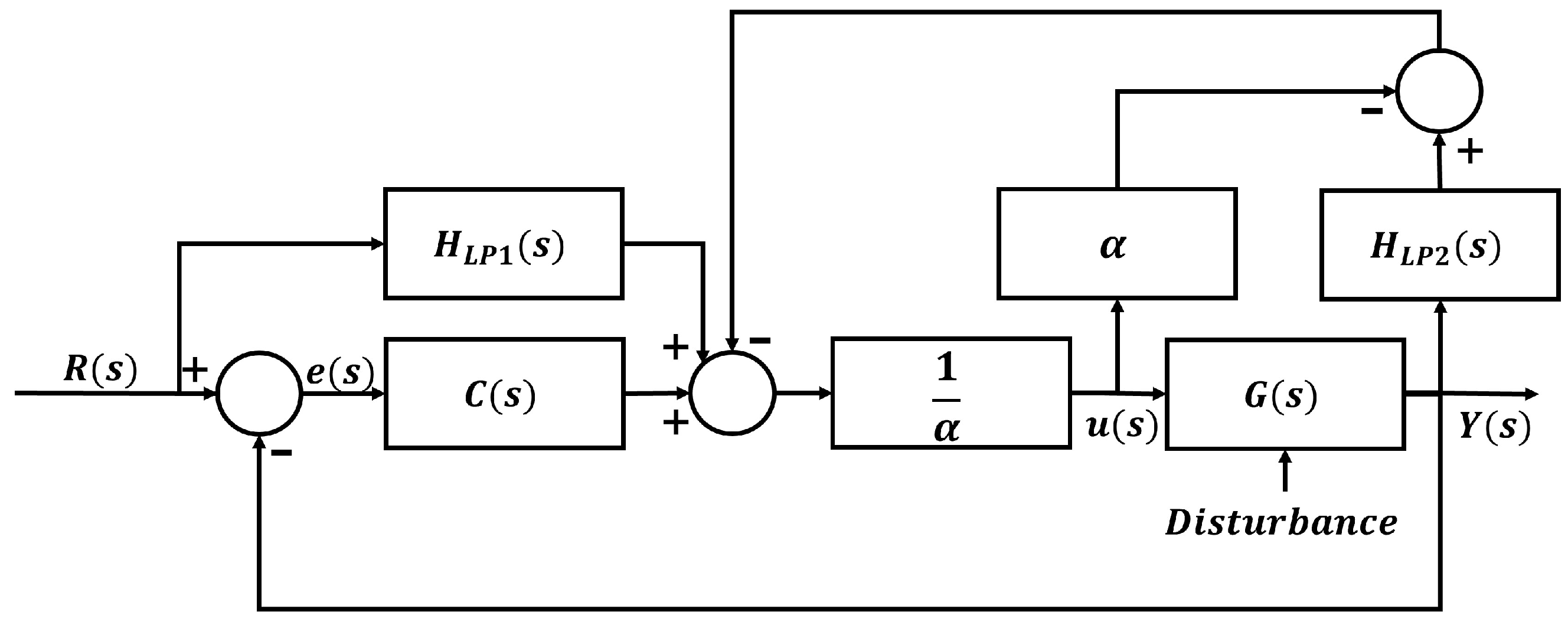
Figure 2 shows the schematic of the implemented iPI controller, where e ( s ) is the tracking error (Equation (8)), C ( s ) is the PI controller, u ( s ) is the control output (Equation (9)), and G ( s ) the greenhouse digital twin (Equations (5) and (6)).
To enable real-time implementation of Model-Free Control, the numerical differentiation required by the ultra-local model must be regularized. Since pure derivatives amplify noise, two first-order low-pass filters, H L P 1 ( s ) and H L P 2 ( s ) , are introduced to approximate the derivatives of the reference R ( s ) and output y ( s ) , respectively.
These filters attenuate high-frequency noise while preserving the signal dynamics needed for effective control. As a result, the estimated derivatives R ˙ ( s ) and y ˙ ( s ) used in F ^ ( s ) (Equation (12)) remain smooth and reliable. Additionally, the 1 / α gain ensures a properly scaled and responsive control action.

3.2. Parameter Optimization Using Genetic Algorithm

MFC strategies lack analytical formulas for direct gain computation, complicating optimal tuning. To address this, following [15], Genetic Algorithms (GA) are employed as a robust model-free optimization method to determine suitable controller parameters. This study adopts the Integral of Squared Error (ISE) and the Integral of Squared Control Output (ISCO) as the cost function, balancing tracking accuracy and control effort:
C f = I S E + I S C O
The GA optimized the initial parameters of the iPI controller and the coefficient α while keeping derivative filter parameters H L P 1 and H L P 2 fixed to reduce dimensionality and preserve numerical stability. These filters attenuate high-frequency noise and have limited influence on overall performance. The gains of each derivative are K L P 1 = K L P 2 = 1 and T L P 1 = T L P 2 = 2 .
The optimal values obtained for the iPI and PI controllers using the genetic algorithm are as follows: for temperature control, the iPI controller parameters are K P T = 18.23 , K I T = 0.361 , and α T = 1 , while the PI controller parameters are K P T = 4.389 and K I T = 0.086 ; for humidity control, the iPI controller parameters are K P W = 19.266 , K I W = 0.108 , and α W = 0.5 , whereas the PI controller parameters are K P W = 6.327 and K I W = 0.031 . The α coefficient, used exclusively in the MFC approach, is not employed by the PI controller.

4. Hardware-in-the-Loop Implementation

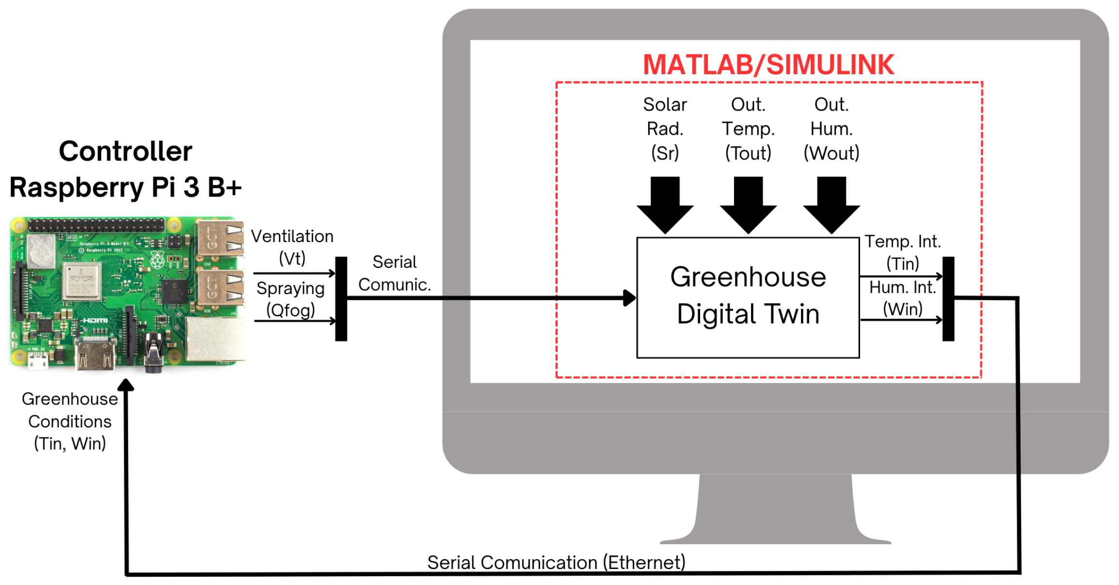
The Hardware-in-the-Loop implementation was developed to evaluate the proposed control strategy in a realistic and safe testing environment [11]. The architecture includes the following: (1) a Raspberry Pi 3 Model B+ executing the controller in real time, and (2) a digital twin of the greenhouse climate dynamics based on the model in Section 2, developed in MATLAB/Simulink R2025b (Figure 3).
The controller and DT communicate via UDP over a local network, allowing real-time exchange of control signals. The DT uses a multivariable continuous-time model discretized with a fixed-step solver to synchronize with the embedded controller.

4.1. Sampling Time for Digital Controller

The selection of sampling time is critical in digital control, especially for strategies like MFC that rely on numerical derivative estimation. As per the Nyquist–Shannon theorem, the sampling rate must be at least twice the highest frequency in the continuous-time system.
In this study, the simulator solves the DT equations and transmits the results to the digital controller, which computes control actions and sends them back. Communication occurs via serial protocol, so the sampling time is limited by transmission speed and the greenhouse’s inherently slow dynamics. A plant sampling time of T s , D T = 1   s was selected.
Following this, the controller sampling time was set according to the Nyquist– Shannon criterion:
T s , c o n t r o l l e r T s , D T 2 = 0.01   s

4.2. Conversion of Designed Controllers from a Continuous System to a Discrete System

The controller was originally designed in the continuous-time domain. However, for HIL implementation, it must be converted to a discrete-time form. According to [16], this is possible by selecting an appropriate sampling time (see Section 4.1) and applying a discretization method, such as the Tustin (trapezoidal) approximation, defined by the following:
s = 2 T s · z 1 z + 1
This method was applied to the H L P filters in the controller to express the derivatives of R ( t ) and y ( t ) in discrete time.
Additionally, the integral gains were adjusted to account for the controller’s sampling period, ensuring equivalent behavior between the continuous and discrete domains:
K I , discrete = K I · T s , controller
This conversion preserves the integral action’s effect in the digital implementation.

5. Results and Discussion

This section presents the response of the MFC iPI controller, implemented on the Raspberry Pi 3 Model B+, as a digital controller in reference tracking and external disturbance scenarios. It also utilizes cost functions to compare its performance with that of a conventional PI controller.

5.1. Digital Controller on Python

Figure 4 presents the flowchart outlining the programming logic used for the MFC iPI controller. The same implementation structure was applied to the traditional PI controller used for comparison.

5.2. Reference Tracking and Disturbance

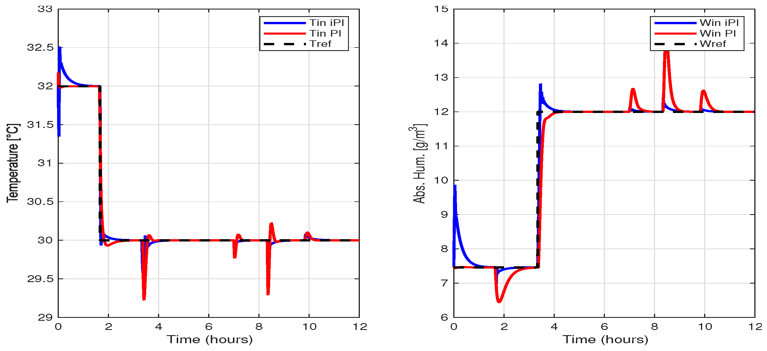
The controllers were evaluated in a 12 h test divided into two phases. In the first 6 h, step changes were applied to the reference signals of T i n and W i n .
As both strategies lack decoupling mechanisms, changes in one reference affect the other variable. The PI controller shows strong coupling—alterations in temperature reference notably impact humidity, and vice versa. The MFC iPI controller, although slower to converge initially, reacts rapidly and accurately once reference changes occur. While some interaction between T i n and W i n persists under the MFC iPI, cross-effects are significantly reduced compared to the PI. Tracking performance is illustrated in Figure 5.
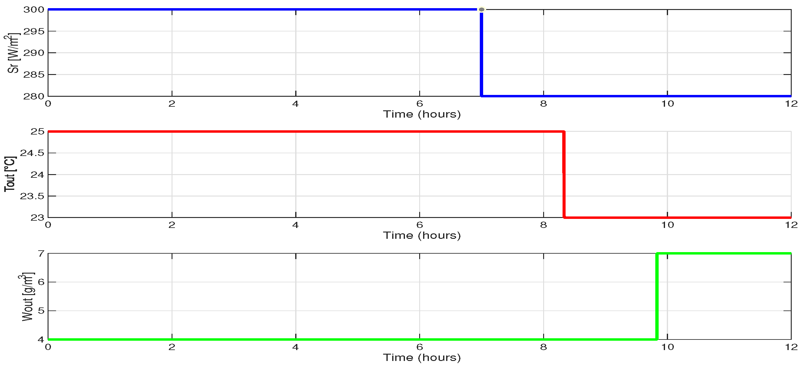
In the second phase, starting at hour 6, external disturbances—solar radiation ( S r ), outdoor temperature ( T o u t ), and humidity ( W o u t )—were introduced (Figure 6).
The PI controller shows poor disturbance rejection, with notable fluctuations in internal variables. Conversely, the MFC iPI maintains stable regulation of T i n and W i n , demonstrating higher robustness to external changes.

5.3. Analysis of Performance Controller

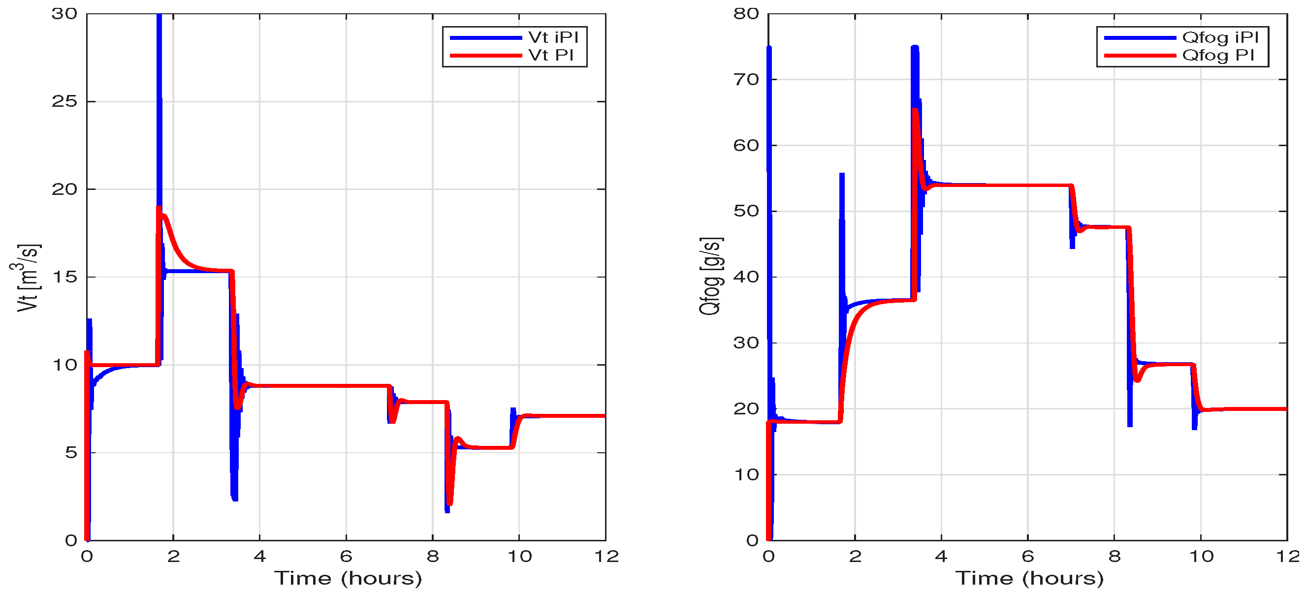
Figure 7 illustrates the behavior of the ventilation rate V t and the fogging flow rate Q f o g . In both cases, the MFC iPI (blue) responds more aggressively to sudden changes in reference or external conditions, exhibiting sharp transients and higher frequency oscillations immediately after a step input. This behavior reflects the high reactivity of the MFC strategy, particularly due to its real-time derivative estimation and the absence of an internal model.
In contrast, the conventional PI controller (red) produces smoother transitions with slower rise times, resulting in more conservative control actions. Despite the initial peaks observed in the MFC iPI response, both controllers eventually converge to similar steady-state values.
Finally, to quantify the performance and control effort of both the MFC iPI and conventional PI controllers, the ISE and ISCO criteria were used. The resulting values for each controller are summarized in Table 1.

6. Conclusions

This study validates the effectiveness of a model-free iPI control strategy embedded in a HIL framework for greenhouse climate regulation. The use of a Raspberry Pi as a real-time controller interacting with a digital twin proved to be a cost-effective and practical solution, enabling realistic testing under operational constraints. The results confirm the robustness, ease of implementation, and adaptability of the model-free approach, even in the absence of accurate process models. Nevertheless, it must be acknowledged that the validation was limited to HIL simulation, and no experiments were conducted in a physical greenhouse, which is planned for future work. Consequently, actuator delays, sensor noise, and plant physiological responses were not directly evaluated, representing a limitation. Moreover, the integration of embedded control, real-time communication, and simulation via DT exemplifies a functional CPS architecture tailored for smart agriculture. This framework facilitates safe pre-deployment evaluation and offers a promising platform for future extensions, including experimental testing in real greenhouse environments, as well as the development of adaptive control, multivariable regulation, and integration with IoT and sensor networks in smart agriculture contexts.

Author Contributions

Conceptualization, A.M., S.V., D.C. and O.C.; methodology, A.M., S.V., D.C. and O.C.; validation, A.M. and O.C.; investigation, A.M., S.V., D.C. and O.C.; writing—original draft preparation, A.M., S.V., D.C. and O.C.; writing—review and editing, A.M., S.V., D.C. and O.C.; supervision, D.C. and O.C.; All authors have read and agreed to the published version of the manuscript.

Funding

Universidad San Francisco de Quito supported this work through the Poli-Grants Program under Grant 33603.

Institutional Review Board Statement

Not applicable.

Informed Consent Statement

Not applicable.

Data Availability Statement

Data are available on request from the authors.

Conflicts of Interest

The authors declare no conflicts of interest.

References

  1. Cevallos, G.; Herrera, M.; Jaimez, R.; Aboukheir, H.; Camacho, O. A practical hybrid control approach for a greenhouse microclimate: A hardware-in-the-loop implementation. Agriculture 2022, 12, 1916. [Google Scholar] [CrossRef]
  2. Albright, L.D.; Arvanitis, K.; Drysdale, A. Environmental control for plants on earth and in space. IEEE Control. Syst. Mag. 2001, 21, 28–47. [Google Scholar]
  3. Faramarzpour, H.; Ghaderi, M.; Reddick, C.; Sorin, M.; Grégoire, M. Specification of a greenhouse in cold climate condition, mathematical model and optimization. J. Build. Phys. 2025, 48, 579–608. [Google Scholar] [CrossRef]
  4. Kimball, B. Simulation of the energy balance of a greenhouse. Agric. Meteorol. 1973, 11, 243–260. [Google Scholar] [CrossRef]
  5. Subin, M.C.; Singh, A.; Kalaichelvi, V.; Karthikeyan, R.; Periasamy, C. Design and robustness analysis of intelligent controllers for commercial greenhouse. Mech. Sci. 2020, 11, 299–316. [Google Scholar] [CrossRef]
  6. Fliess, M.; Join, C. Model-free control. Int. J. Control. 2013, 86, 2228–2252. [Google Scholar] [CrossRef]
  7. Precup, R.E.; Radac, M.B.; Roman, R.C.; Petriu, E.M. Model-free sliding mode control of nonlinear systems: Algorithms and experiments. Inf. Sci. 2017, 381, 176–192. [Google Scholar] [CrossRef]
  8. Vega, S.; Iza, J.; Cruz, W.; Gude, J.J.; Camacho, O. A Comparative Experimental Evaluation of iPI and iPI-Fuzzy Controllers for a Thermal Process with a Long Dead Time. In Proceedings of the 15th International Conference on Simulation and Modeling Methodologies, Technologies and Applications (SIMULTECH 2025), Bilbao, Spain, 11–13 June 2025; pp. 209–216. [Google Scholar]
  9. Lafont, F.; Pessel, N.; Balmat, J.F.; Fliess, M. On the model-free control of an experimental greenhouse. Comput. Electron. Agric. 2015, 110, 139–149. [Google Scholar] [CrossRef]
  10. Seol, J.; Park, Y.; Pak, J.; Jo, Y.; Lee, G.; Kim, Y.; Ju, C.; Hong, A.; Son, H.I. Human-Centered Robotic System for Agricultural Applications: Design, Development, and Field Evaluation. Agriculture 2024, 14, 1985. [Google Scholar] [CrossRef]
  11. Cevallos, G.; Pinzón, J.; Camacho, O. A Microclimate Greenhouse Multivariable Control: A Guide to use Hardware in the Loop Simulation. In Proceedings of the 2022 IEEE International Conference on Automation/XXV Congress of the Chilean Association of Automatic Control (ICA-ACCA), Curico, Chile, 24–28 October 2022; IEEE: Piscataway, NJ, USA, 2022; pp. 1–6. [Google Scholar]
  12. Lakshmi, A.J.; Dasari, R.; Chilukuri, M.; Tirumani, Y.; PramodKumar, A. IoT Based Smart Greenhouse Using Raspberry Pi. In Proceedings of the 2023 International Conference on Computer, Electronics & Electrical Engineering & their Applications (IC2E3), Garhwal, India, 8–9 June 2023; IEEE: Piscataway, NJ, USA, 2023; pp. 1–6. [Google Scholar]
  13. Pasgianos, G.; Arvanitis, K.; Polycarpou, P.; Sigrimis, N. A nonlinear feedback technique for greenhouse environmental control. Comput. Electron. Agric. 2003, 40, 153–177. [Google Scholar] [CrossRef]
  14. Giraldo, S.A.C.; Flesch, R.C.; Normey-Rico, J.E. Multivariable greenhouse control using the filtered smith predictor. J. Control. Autom. Electr. Syst. 2016, 27, 349–358. [Google Scholar] [CrossRef]
  15. Hu, H.; Xu, L.; Wei, R.; Zhu, B. Multi-objective control optimization for greenhouse environment using evolutionary algorithms. Sensors 2011, 11, 5792–5807. [Google Scholar] [CrossRef] [PubMed]
  16. Rubio-Díaz-Cordovés, Á.; Gil-Nobajas, J.J. Fundamentos de Control Automático de Sistemas Continuos y Muestreados; Universidad de Navarra, Escuela Superior de Ingenieros: San Sebastián, España, 2009; ISBN 978-84-613-4618-9. Available online: https://www.euskariana.euskadi.eus/euskadibib/eu/bib/1157906.do (accessed on 2 August 2025).
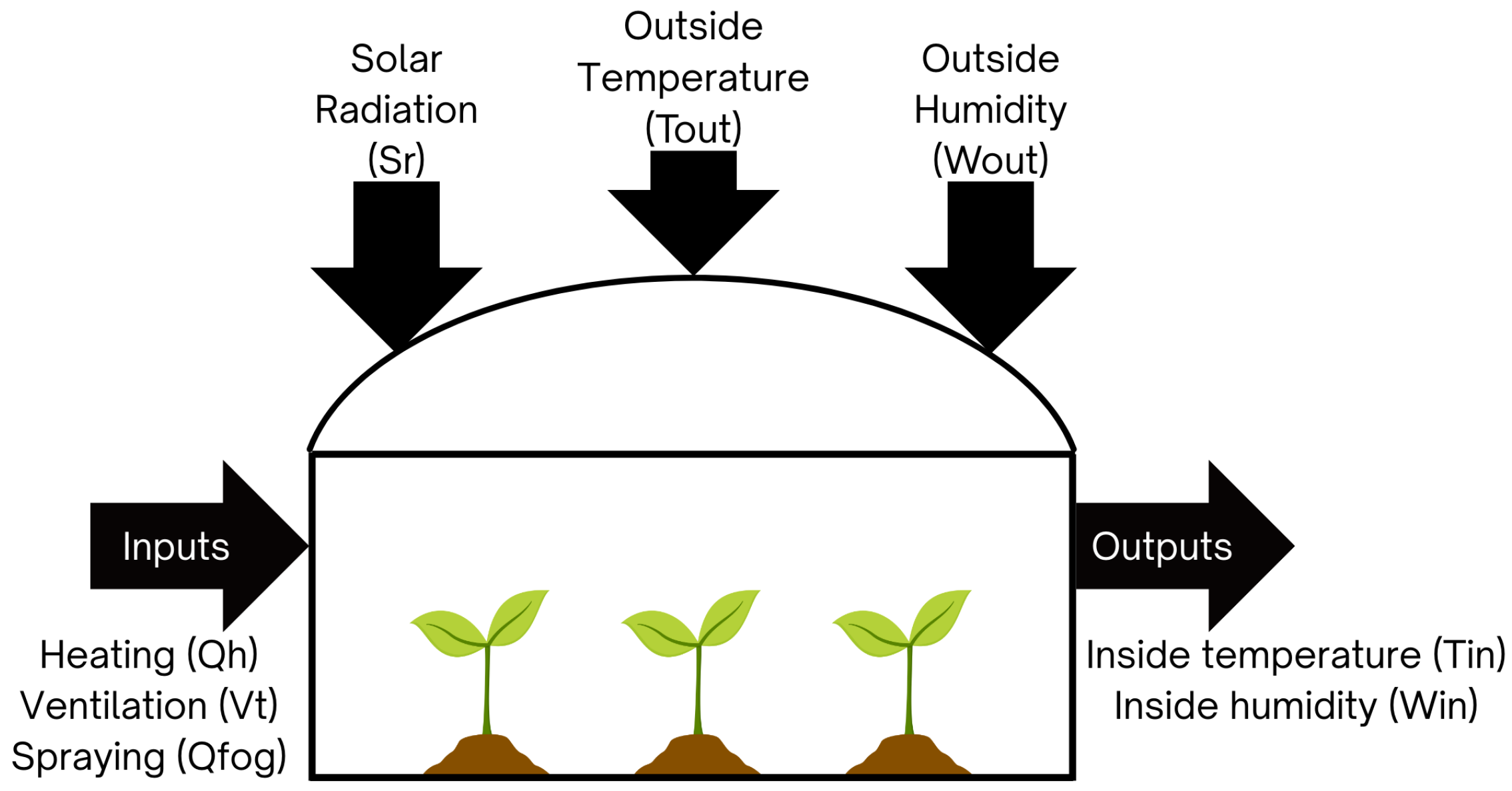
Figure 1. Greenhouse schematic with inputs, outputs, and disturbances.
Engproc 115 00015 g001
Figure 2. Schematic of MFC structure.
Engproc 115 00015 g002
Figure 3. Hardware-in-the-Loop implementation.
Engproc 115 00015 g003
Figure 4. Flowchart of the programming logic implemented for the MFC iPI and traditional PI on Python 3.7.3 (Python Software Foundation, Wilmington, DE, USA).
Engproc 115 00015 g004
Figure 5. Tracking performance of the T i n and W i n using the MFC iPI and PI.
Engproc 115 00015 g005
Figure 6. External disturbances applied to the greenhouse digital twin during the experiment: Solar radiation S r , outdoor temperature T o u t , and outdoor humidity W o u t .
Engproc 115 00015 g006
Figure 7. Control actions for ventilation rate V t and fogging flow rate Q f o g generated by the MFC iPI and PI controllers in the T i n and W i n loops, respectively.
Engproc 115 00015 g007
Table 1. Optimized parameters of the controllers obtained using the GA.
Performance IndieiPIPI
ISE V t 1.492   ×   10 11 1.557  ×   10 11
ISE Q f o g 2.501  ×   10 12 2.49  ×   10 12
ISCO V t 5.812  ×   10 4 9.766  ×   10 3
ISCO Q f o g 3.55  ×   10 6 1.234  ×   10 5
Disclaimer/Publisher’s Note: The statements, opinions and data contained in all publications are solely those of the individual author(s) and contributor(s) and not of MDPI and/or the editor(s). MDPI and/or the editor(s) disclaim responsibility for any injury to people or property resulting from any ideas, methods, instructions or products referred to in the content.