Dynamical Modeling of Floods Using Surface Water Level Time Series ^†

Abstract

We present a dynamical systems approach to modeling nonlinear flood dynamics using 20 years of water level data from Durazno, Uruguay. Flood events are identified, and their periodicity and temporal distribution are analyzed in relation to rain gauge precipitation. Phase space reconstruction enables data-driven neural network modeling and quantification of the relationship between water level and soil moisture. Bifurcation diagrams define basin-specific flood thresholds, offering a mechanistic framework for improved flood forecasting and risk assessment.

1. Introduction

Floods represent one of the most frequent and devastating hazards globally, causing significant loss of life, economic damage, and alteration to ecosystems and communities. Accurate prediction and risk assessment remain challenging due to the inherently complex, nonlinear dynamics governing flood generation processes within river basins. Traditional hydrological models often struggle to fully capture this complexity, particularly the intricate interplay between precipitation, antecedent catchment conditions like soil moisture, and resulting water levels [1,2].

In regions susceptible to recurrent flooding, understanding these dynamics is crucial for effective water resource management and disaster mitigation. While statistical and physically based models offer valuable insights, approaches grounded in dynamical systems theory provide a powerful alternative framework for analyzing the underlying chaotic or nonlinear behavior inherent in hydrological time series [3,4]. We leverage 20 years of daily water surface level data from Durazno, Uruguay. The goal of this work is to identify and characterize flood events and their temporal patterns using data-driven neural networks within the reconstructed phase space. A dynamical system to quantify the relationship between river levels and antecedent soil moisture derived from rainfall was employed. In addition, bifurcation diagrams to define basin-specific flood thresholds as a function of accumulated rain were used.

2. Materials and Methods

2.1. Study Area

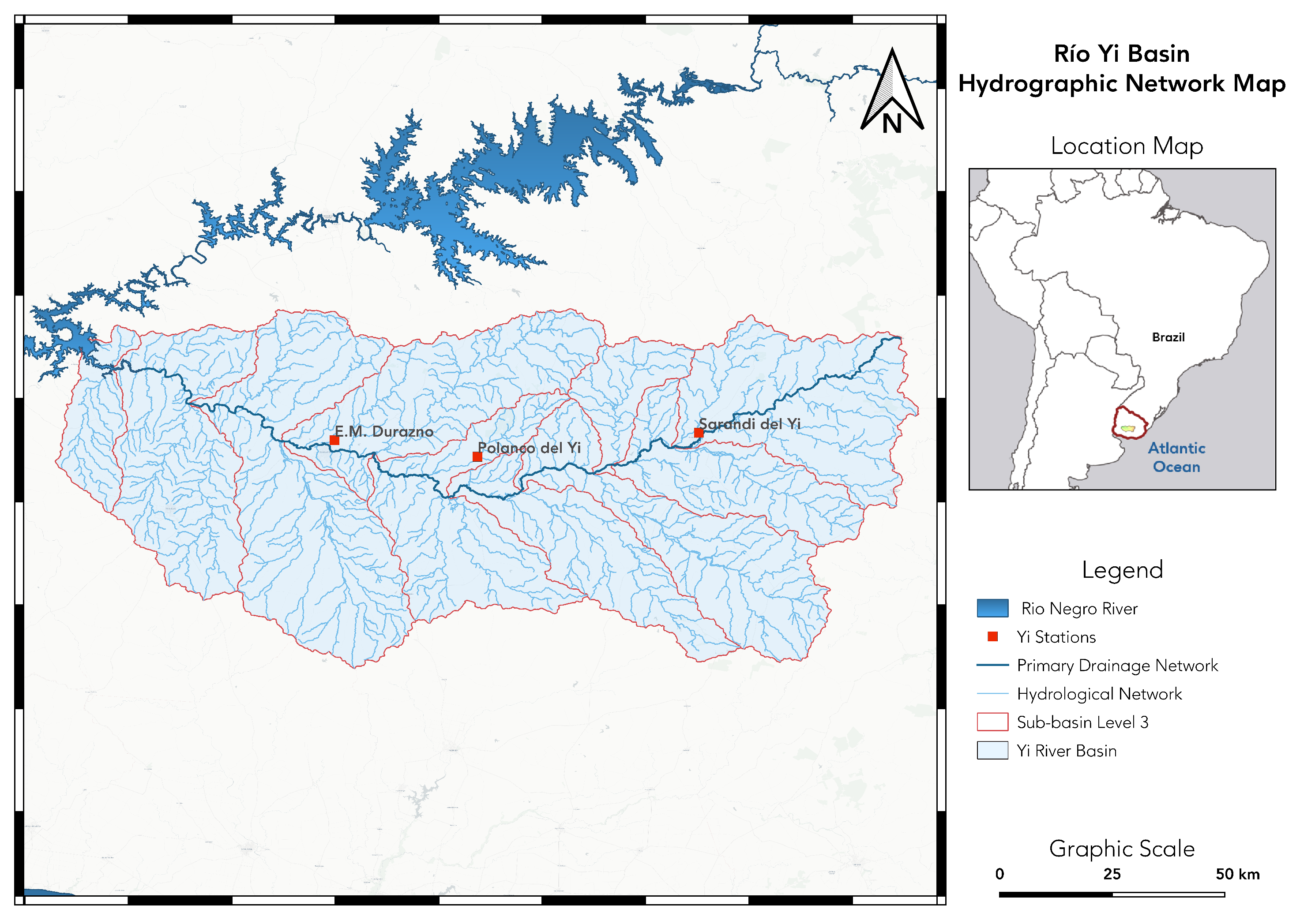
The Yi River basin has a total area of 13,621.50 km², and represents approximately 18.55% of the total Negro River basin. The Yi River basin covers an area of 8900 km² upstream of the city of Durazno. The channel length, from its headwaters to the city, is 192 km, with a gradient of 0.12%, resulting in a concentration time of 52 h [5]. This study was based on hydrological events that occurred in the study area during the years 2007, 2010, 2015, 2016, 2019, 2020, and 2024 (https://goo.su/PuGQlDt (accessed on 10 February 2025)).

2.2. Hydrological Data

The time series of water level and rain gauge precipitation covers the period from 1 January 2006 to 31 December 2024. The selected period includes extreme precipitation events that caused flooding. The dataset was obtained from the hydrometric monitoring stations of the National Administration of Power Plants and Transmission (UTE (https://www.ute.com.uy/institucional/ute/utei/precipitaciones-y-prevision-de-niveles (accessed on 15 February 2025)). Figure 1 shows the spatial locations of the hydrometeorological monitoring stations that were used for the implementation of the flood models for the Durazno station.

3. Hydological Modeling

Considering that a watershed can be divided into N sub-watersheds in series, the linear cascade, originally proposed by Nash (1970), is a series of linear reservoirs arranged in such a way that the output from the upstream reservoir is used as the input to the downstream reservoir in the form of a cascade [1,6].

$${\displaystyle \frac{dh}{dt}}=i\left(t\right)-q\left(t\right)$$

(1)

where $h\left(t\right)$ is the surface water height; $i\left(t\right)$ are the contributions of water to the system, such as precipitation and runoff; and $q\left(t\right)$ are the output flows, such as overflows and infiltration.

The flow–volume relationship in a channel can be determined using the hydraulic relationship

$$q\left(t\right)=cv{\left(t\right)}^n$$

(2)

known as Manning’s law [1,2,7], where c is a parameter that includes terrain properties, roughness, and geometry, and n is an exponent related to the system, typically $n=1/2$ for linear systems.

The factors that contribute the most to a flood are intense rainfall in short periods of time. In addition, the most important outflows are the surface flow and the infiltration of water into the soil. Considering the infiltration as the variable infiltration capacity (VIC), the model assumes that the infiltration capacity, defined as the maximum depth of water that can be stored in the soil column, and therefore runoff generation and evapo-transpiration, vary within an area (grid cell or catchment) due to variations in topography, soil, and vegetation [8].

The variation in infiltration capacity I over an area is expressed as

$$I=i_{max}(1-{\displaystyle \frac{(1-A)}{\beta }})$$

(3)

where A is the fraction of a grid cell area for which the infiltration capacity is less than I $(0\le A\le 1)$, $i_{max}$ is the maximum infiltration capacity within the grid cell [mm], and $\beta$ is the infiltration shape parameter, which is a measure of the spatial variability of the infiltration capacity. The VIC model assumes that surface runoff (direct flow) is generated by those areas for which precipitation, when added to the soil moisture storage at the end of the previous time step, exceeds the storage capacity of the soil. When the soil is saturated, the drainage term follows the saturated hydraulic conductivity [2].

We can formulate a simple model to represent the surface water level dynamics in a given hydrological system using the following equation:

$${\displaystyle \frac{dh\left(t\right)}{dt}}=r\left(t\right)-I\left(t\right)-q\left(t\right)$$

(4)

Similarly, let us establish a differential equation to model the dynamics of soil saturation:

$${\displaystyle \frac{ds\left(t\right)}{dt}}=I\left(t\right)-\alpha s\left(t\right)$$

(5)

where $\alpha$ is the natural soil drainage rate.

3.1. A Dynamic Model for Floods

Using (4) and (5), let us construct a dynamical system as follows:

$$\left\{\begin{array}{c}{\displaystyle \frac{dh\left(t\right)}{dt}}=r\left(t\right)-I\left(t\right)-q\left(t\right)\hfill \\ {\displaystyle \frac{ds\left(t\right)}{dt}}=I\left(t\right)-\alpha s\left(t\right)\hfill \end{array}\right.$$

(6)

From the point of view of dynamical systems, a physical system can be generally represented as follows [9]:

$$\dot{\mathbf{x}}=\mathbf{f}(\mathbf{x}\left(t\right),\mathbf{u}\left(t\right),\mathbf{p}),\mathbf{x}\left(0\right)={\mathbf{x}}_{\mathbf{0}}$$

(7)

where $\mathbf{x}\left(t\right)$ is a vector of states of the system at a given time, $\mathbf{u}\left(t\right)$ is a vector of external inputs such as precipitation, and $\mathbf{p}$ is the system parameters. The central aim in a dynamical system is to identify $\mathbf{f}$, which is a nonlinear function that describes the rates of change of the state variables. In this sense, we propose, based on hydrological time series, that $\mathbf{f}$ can be approximated based on two approaches: first using an embedding dimension method, and then using a data-driven approach involving a model based on neural networks differential equation approach [4,10,11].

3.2. Neural Network Surrogate Model

The general idea of an artificial neural network is to find a model that, based on a set of N samples

$$D=\left\{\right|x_1,...,x_N|,|y_1,...,y_N\left|\right\}$$

(8)

will approximate an unknown function f, with

$$f\left(x_i\right)=y_i$$

(9)

as well as possible.

Theorem 1.

A feedforward neural network with a single hidden layer and a finite number of neurons can approximate any continuous function on a compact subset of the real numbers.

Let $C\left(K\right)$ be the space of continuous functions on a compact set $K\subseteq R^n$. For any continuous function $f\in C\left(K\right)$ and for any $ϵ>0$, there exists a neural network $\widehat{f}$ with a single hidden layer, such that

$$|f\left(x\right)-\widehat{f}\left(x\right)|<ϵforx\in K$$

(10)

This means that the neural network $\widehat{f}\left(x\right)$ can approximate the function $f\left(x\right)$ to within any arbitrary degree of accuracy ϵ.

The functional form of the ANN-based model is a linear combination of fixed-basis functions:

$$f_k(\mathbf{x},\mathbf{w})=\sigma \{\sum _{j=1}^M{w}_{kj}^{\left(2\right)}y(\sum _{j=1}^D{w}_{ji}^{\left(1\right)}{\mathbf{x}}_{\mathbf{i}}+w_{j0}^{\left(1\right)})+w_{k0}^{\left(2\right)}\}.$$

(11)

where the map $\sigma (.)$ is a nonlinear activation function. The ANN goal is to extend this model by making the basis functions ${\varphi }_j\left(\mathbf{x}\right)$ depend on parameters, and then to allow these parameters to be adjusted along the coefficients $\left\{w_j\right\}\in \mathbf{w}$ during the training. In Equation (11), each basis function is itself a nonlinear function of linear combinations of the inputs, where the coefficients in the linear combination are adaptive parameters. In other words, an ANN model can be described as a series of functional transformations. We can combine these various stages to give the overall network function that, for any $\sigma (.)$, outputs unit activation functions.

3.3. Model Evaluation

The neural network surrogate model was evaluated with two metrics: Nash–Sutcliffe efficiency (NSE) and Root Mean Squared Error (RMSE), as well as visual criteria for the observed and simulated levels, the RMSE is calculated using the following equation:

$$RMSE=\sqrt{{\displaystyle \frac{1}{N}}{\displaystyle \sum _{i=1}^N}{(h\left(t_i\right)-\widehat{h}\left(t_i\right))}^2}.$$

(12)

NSE efficiency is a value between ($-\infty ,1$). Values of the NSE nearer to 1, suggest a model with more predictive skill [6]. It is defined as:

$$NSE=1-{\displaystyle \frac{{\sum }_{i=1}^N{(h\left(t_i\right)-\widehat{h}\left(t_i\right))}^2}{{\sum }_{i=1}^N{(h\left(t_i\right)-\overline{h}\left(t_i\right))}^2}}.$$

(13)

where $h\left(t_i\right)$ is the observed value, $\widehat{h}\left(t_i\right)$ is the predicted value and $\overline{h}\left(t_i\right)$ is the mean of the observed water level.

4. Results

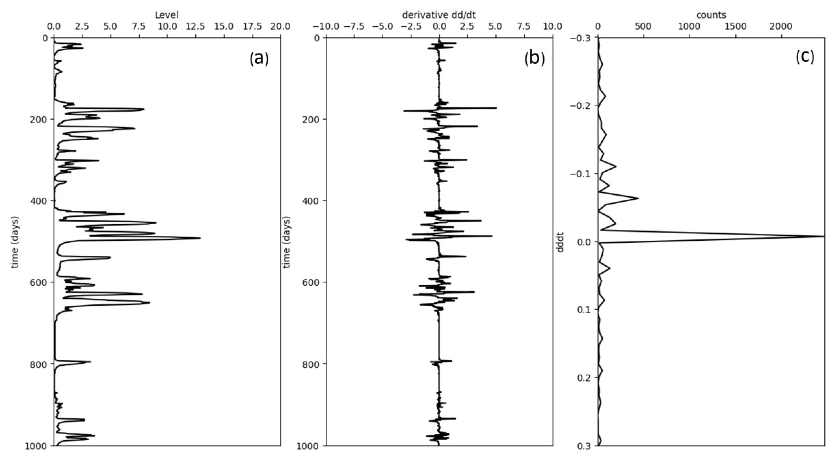
Figure 2 (left) displays a dataset containing multiple periods of high water levels, corresponding to floods caused by rainstorms in the Río Yi basin, Uruguay. Most storm events exhibit an asymmetric pattern, characterized by a rapid rise followed by a slower decline. This asymmetry arises because the river level increases quickly at the onset of rainfall, but recedes gradually as water drains from the land slowly.

The rate curve, shown in the middle of Figure 2, reveals numerous short events, which appear two-sided in shape. Given that a typical storm event consists of a sharp rise followed by a prolonged decline, we expect negative level rates to be more frequent than positive ones. Figure 2 (right) confirms, with the histogram peaks at negative rates, that storm events are typically asymmetric.

Figure 3 shows scatter plots of the samples lagged at 1, 3, and 30 days based on the embedding phase space reconstruction method. The loss of correlation and the nonlinear character of the time series can be observed. The Lyapunov exponent analysis yielded the following results: $0.3018,0.0678,-0.0978,-0.3331$; these values gives indications of the stochastic character and the level time series [9,12].

4.1. Dynamical System Results

The flood model based on dynamical systems involves setting up differential equations that capture key hydrological processes, analyzing equilibria and stability, and studying how changes in parameters like rainfall intensity or inputs lead to flooding conditions. The complexity can be adjusted depending on the desired level of detail and whether spatial components are included. The study of equilibrium solutions allowed us to determine solutions for the variables h and s as a function of the rain, as well as soil properties such as infiltration.

Theorem 2.

The dynamical system (6) has an equilibrium solution $(h_0,s_0)$ such that $(h_0,s_0)>0$.

The demonstration follows from the properties of the resulting functions from solve the equilibrium points ${\displaystyle \frac{dh\left(t\right)}{dt}}=0,{\displaystyle \frac{ds\left(t\right)}{dt}}=0$.

The bifurcation diagram for a flood model based on differential equations is shown on the left side of Figure 4, considering the river level and soil saturation as relevant variables, thus allowing the determination of critical flood values based on observed rainfall patterns. In addition, it is possible to determine the increase in the surface water level as a function of time for a given rainfall condition, as shown on the right side of Figure 4, based on the equilibrium solutions from Theorem 2.

This result shows the possibility of modeling different flood contexts based on the physical characteristics of the basin, such as concentration time and soil infiltration properties. The results shows the value of the surface water level that could be reached under a given situation [13].

4.2. Results of Neural Network Surrogate Model

In order to estimate the function f that describes the dynamics of the system in (7), we propose a Long Short Term Memory neural network topology with a Rectified Linear Unit (ReLu) activation function, given by $\sigma =Relu\left(\mathbf{x}\right)=max(\mathbf{x},0)$. This was employed with the aim of activating the neurons with the maximum values of the series, since they correspond to the maximum level events in different training periods. For this period, the neural network model also included, as input, rain gauge data that have been extracted from hydrometric stations. The input dataset for model conditioning was split into $70\%$ for training and $30\%$ for validation. The loss function adopted for the network was the mean absolute error (MAE) and the Adam optimizer. The historical level and rain data of the stations were analyzed to estimate the future river level and evaluate the model until all the network hyperparameters had been calibrated.

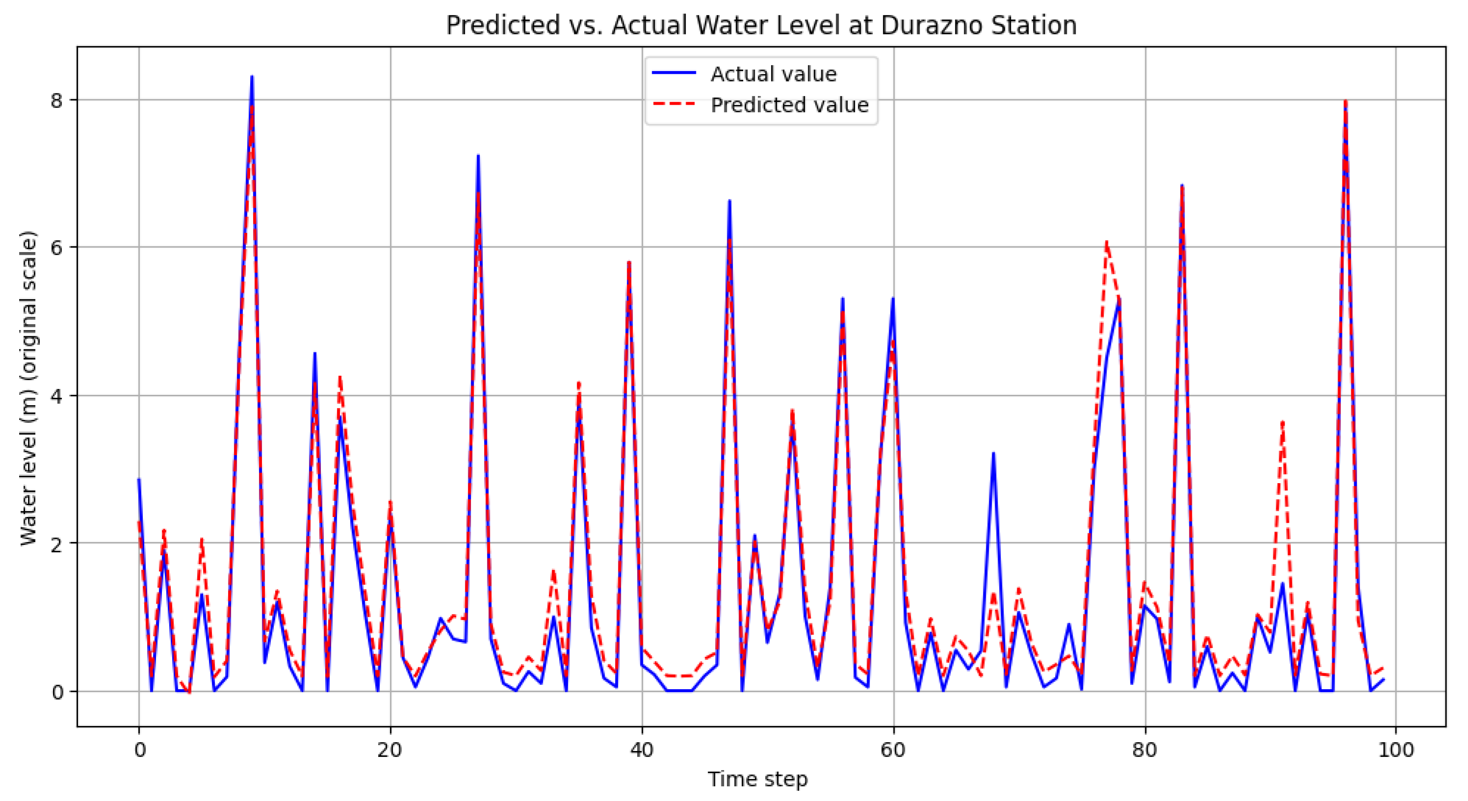
Figure 5 shows the results of the model for predicting river level time series for the lowest station in the basin, Durazno. The time series predicted by the model in the testing period for one day are presented in Figure 5. It is possible to observe the accuracy of the model for predictions for one day with different input configurations; it shows good performance according to the evaluation metrics. Another possible result that could be obtained from the neural network is the discharge at a specific point in the river, which would allow for the determination of discharges at points where there are no flow curves, another hydraulic parameter of interest in the study of floods.

5. Conclusions

This study integrates dynamical systems and data-driven neural network approaches to model flood dynamics in the Yi River basin, demonstrating their complementary strengths in enhancing flood prediction accuracy and interpretability. The dynamical systems framework, through differential equations and bifurcation analysis, provides a mechanistic understanding of flood generation by capturing nonlinear interactions between rainfall, soil moisture, and surface water levels. This approach enables the identification of critical thresholds and equilibrium states, offering a robust theoretical foundation for flood forecasting. Conversely, the LSTM-based neural network surrogate model excels in leveraging historical time series data to predict river levels with high precision, achieving a Nash–Sutcliffe Efficiency (NSE) of $0.97$ and a Root Mean Square Error (RMSE) of $1.6\%$. The neural network’s ability to model complex, nonlinear patterns, particularly during high-rainfall events, complements the physical insights provided by the dynamical system, creating a synergistic framework that balances interpretability with predictive efficiency.

Future work will focus on enhancing model performance by incorporating additional data sources, such as real-time meteorological inputs and spatially distributed soil moisture measurements, to improve flood peak attenuation and prediction accuracy. This hybrid approach underscores the potential of combining physically grounded dynamical systems with data-driven methods to advance flood risk management, particularly in data-scarce regions, providing actionable insights for disaster mitigation and water resource planning.

References

- Wang, G.-T.; Chen, S. A linear spatially distributed model for a surface rainfall-runoff system. J. Hydrol. 1996, 185, 183–198. [Google Scholar] [CrossRef]
- Jayawardena, A.W. Environmental and Hydrological Systems Modelling; Taylor and Francis Group and CRC Press: Boca Baton, FL, USA, 2014; p. 516. [Google Scholar]
- Köhne, J.M.; Wöhling, T.; Pot, V.; Benoit, P.; Leguédois, S.; Le Bissonnais, Y.; Šimůnek, J. Coupled simulation of surface runoff and soil water flow using multi-objective parameter estimation. J. Hydrol. 2011, 403, 141–156. [Google Scholar] [CrossRef]
- Duque, J.S.; Santos, R.; Arteaga, J.; Oyarzabal, R.S.; Santos, L.B. Nonlinear hydrological time series modeling to forecast river level dynamics in the Rio Negro Uruguay basin. Chaos 2024, 34, 053132. [Google Scholar] [CrossRef] [PubMed]
- Luis, S.l.; Christian, C.l.; Magdalena, C.l.; Gabriel, U.l.; Jimena, A. Sistema de alerta temprana para previsión de avenidas en la ciudad de Durazno. Innotec 2015, 10, 56–63. Available online: https://www.redalyc.org/articulo.oa?id=606166715006 (accessed on 10 February 2025).
- Nash, J.; Sutcliffe, J.V. River flow forecasting through conceptual models part i—A discussion of principles. J. Hydrol. 1970, 10, 282–290. [Google Scholar] [CrossRef]
- Zhu, Y.; Zhang, Y.; Yang, J.; Nguyen, B.T.; Wang, Y. A novel method for calculating distributed water depth and flow velocity of stormwater runoff during the heavy rainfall events. J. Hydrol. 2022, 612 Pt A, 128064. [Google Scholar] [CrossRef]
- Gu, H.; Xu, Y.; Ma, D.; Xie, J.; Liu, L.; Bai, Z. A surrogate model for the variable infiltration capacity model using deep learning artificial neural network. J. Hydrol. 2020, 588, 125019. [Google Scholar] [CrossRef]
- Jayawardena, A.W.; Lai, F. Analysis and prediction of chaos in rainfall and stream flow time series. J. Hydrol. 1994, 153, 23–52. [Google Scholar] [CrossRef]
- Kantz, H.; Schreiber, T. Nonlinear Time Series Analysis; Cambridge University Press: Cambridge, UK, 2003. [Google Scholar]
- Kidger, P. On Neural Differential Equations. arXiv 2022, arXiv:2202.02435. [Google Scholar] [PubMed]
- Wolf, A.; Swift, J.B.; Swinney, H.L.; Vastano, J.A. Determining Lyapunov exponents from a time series. Phys. D Nonlinear Phenom. 1985, 16, 285–317. [Google Scholar] [CrossRef]
- Hamzi, B.; Owhadi, H. Learning dynamical systems from data: A simple cross-validation perspective, part i: Parametric kernel flows. Phys. D Nonlinear Phenom. 2021, 421, 132817. [Google Scholar] [CrossRef]