Innovative Elastography Measuring Cap for Ex Vivo Liver Condition Assessment: Numerical and Preclinical Studies in a Porcine Model

Abstract

The authors of this study focused their research on developing cap geometries for the FibroScan^® elastograph (FibroScan, EchoSens, Paris, France) measuring head aimed at a non-invasive assessment of liver condition for transplantation using a pig animal model. Numerical models were created to simulate the propagation of a mechanical wave through a biological medium induced by the FibroScan^® elastograph measuring head. The designed caps were intended to replicate the skin–muscle–rib–liver structures to minimize the risk of damage caused by mechanical wave excitation when directly applied to liver tissue. The construction process of numerical models for the liver and surrounding tissues is presented, along with simulations reflecting the mechanical and acoustic properties of the wave propagation process. The results obtained from in vivo measurements on pigs were validated through a numerical analysis, confirming a high level of agreement between the test results and the numerical model.

1. Introduction

Tools designed for diagnosing the condition of human organs can also be utilized to evaluate the health of livers intended for transplantation. One such device is the FibroScan^® elastograph, which allows for the non-invasive evaluation of the liver by generating mechanical waves and measuring their propagation speed and attenuation using ultrasound. There are two types of ultrasound probes: the M for general applications and the XL which was specifically designed for obese individuals. The test performed with this device is characterized by a high reproducibility of the results, the speed of the process, and a high diagnostic value [1,2].

Liver transplantation studies require non-invasive evaluation methods as existing tests fail to fully meet this need. Liver biopsy currently remains the best method, but it is invasive, and the time needed to analyze the results is lengthy. The FibroScan^® device can be a valuable tool for assessing the condition of the organ before transplantation, particularly due to the limited time available for evaluation [3].

Currently, there is limited studies on the application of transient elastography, including the FibroScan^® device, for assessing liver fibrosis [4]. Studies indicate that the device demonstrates potential effectiveness; however, its performance is significantly limited in patients with obesity. Animal studies, including pig livers, may provide valuable data on the effectiveness of the device and its potential limitations. Attention is drawn to the need for further research to improve the device to allow for a more accurate assessment of the organ’s condition before transplantation.

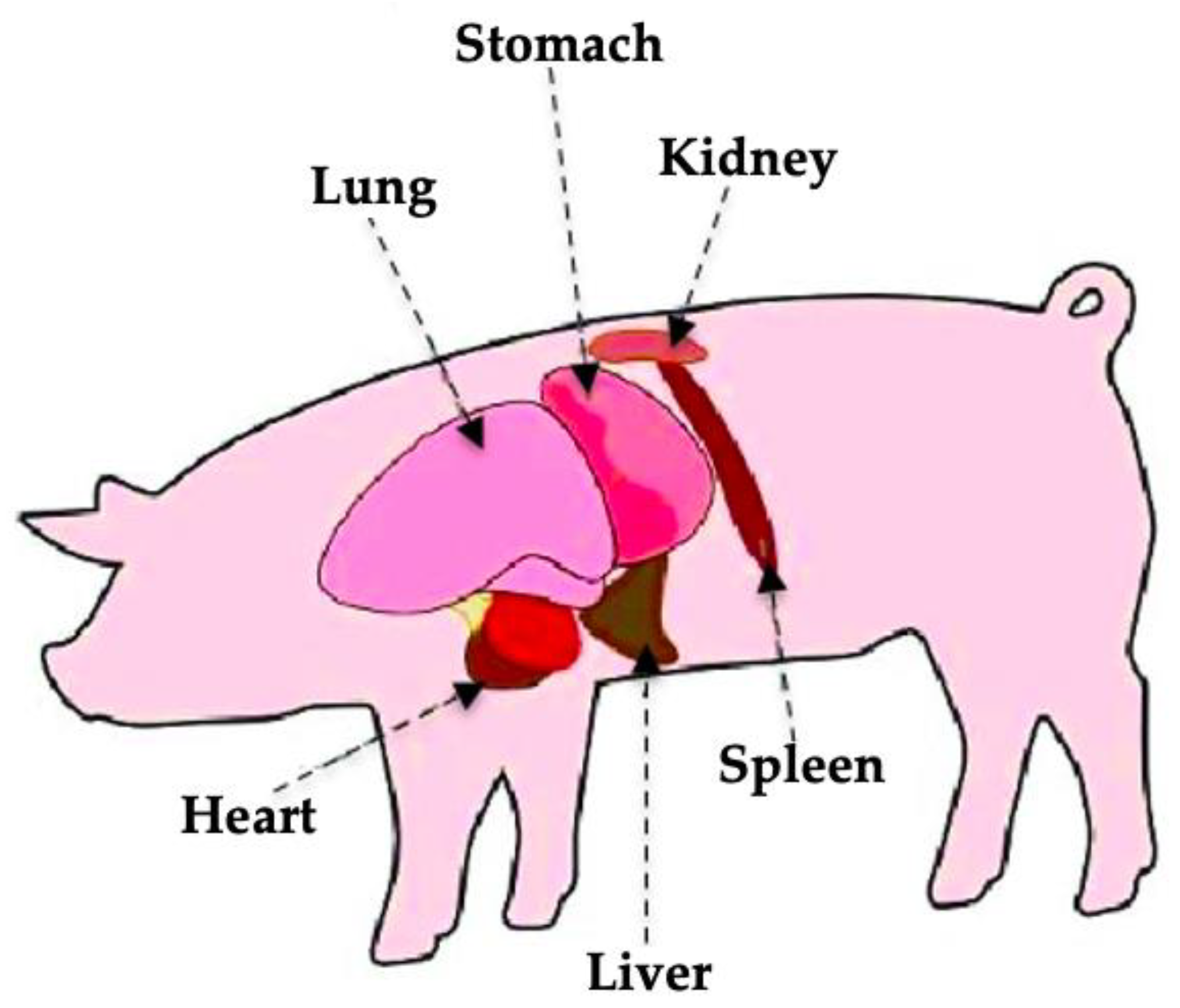
The anatomy of the porcine digestive system shows significant differences from that of humans; nevertheless, the physiology of digestion and, more specifically, the course of digestive processes in both species are similar. Despite the presence of anatomical discrepancies, pigs are a frequently used gastrointestinal model for clinical studies. Figure 1 shows an overview of the distribution of organs in the thorax of the domestic pig. Depending on the age and species, the geometric dimensions of organs such as the liver vary.

A French–German research group conducted a study on “Non-Invasive Assessment of Liver Fibrosis by Vibration-Controlled Transient Elastography (Fibroscan^®)” using fresh pig livers [6]. It has been observed that liver stiffness increases with the rise in shear wave frequency. Consequently, higher frequencies result in greater measured stiffness values. Key findings from the use of the FibroScan^® device include its capability to differentiate between early and advanced cirrhosis, its strong prognostic value for predicting patient survival, and its utility in monitoring patients undergoing treatment. However, the presence of ascites has been identified as a significant physical limitation to elastography, as fluid accumulation obstructs the propagation of shear waves, preventing them from reaching the liver.

A team representing the University of Heidelberg presented a study in the Journal of Hepatology indicating that liver stiffness is directly influenced by central venous pressure [7]. They conducted elastography studies using the Fibroscan^® device for 10 landrace pigs. In their study, liver stiffness was evaluated as a function of venous pressure in an isolated pig liver by clamping the superior and inferior vena cava, the reflux vein, and the hepatic artery. Their findings demonstrated that central venous pressure directly and reversibly regulates liver stiffness. Over a wide range, liver stiffness exhibited a linear relationship with intravenous pressure, reaching an upper detection limit of 75 kPa at an intravenous pressure of 36 cm in a water column. This pronounced dependence of stiffness on venous pressure highlights the necessity of excluding hepatic congestion before assessing fibrosis.

Given the research problem outlined above, the aim of this article is to perform preliminary analyses of mechanical wave propagation within the studied system, specifically the porcine skin–liver system. The primary objective is to achieve satisfactory outcomes through a proposed modification to the measurement head overlay of the FibroScan^® device. This modification is designed to ensure that its application does not cause structural damage to the organ as a result of mechanical wave excitation.

Therefore, it is necessary to develop numerical models that will allow for a rapid preliminary assessment of the propagation of mechanical waves in liver tissue and other relevant parameters. This requires constructing accurate geometric representations of the liver system and incorporating materials that mimic the properties of the skin and adjacent tissues. These models will then be enhanced by applying suitable initial and boundary conditions to replicate the environment observed during in vivo animal experiments.

2. Research Material

2.1. Liver

The liver of the pig is located in the abdominal cavity, on the right side of the body. It occupies most of the abdominal space and is surrounded by other organs. The average weight of the liver in pigs is approximately 1 kg, with its volume ranging between 640 and 910 mL in pigs aged 9 to 12 weeks and weighing between 25 and 35 kg [8].

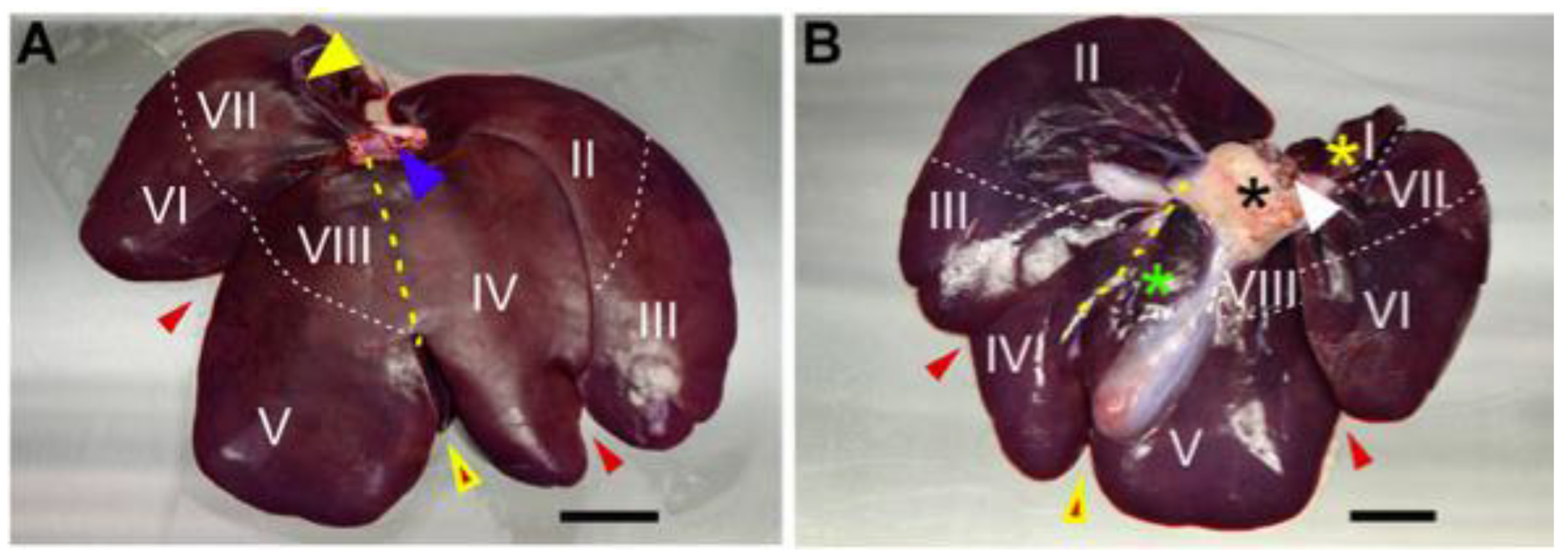
In the structure of the pig liver, 5–6 lobes are distinguished. Their number depends on the breed under consideration. Regardless of the species, their minimum number is always 5, and they are defined as the left lateral, left medial, right lateral, right medial, and caudal lobes. From a ventral perspective, four lobes can be observed in the following order from left to right: left lateral, left medial, right medial, and right lateral. When these are elevated, it is possible to observe the caudal lobe surrounding the vena cava [9]. The sections are separated by deep interlobular fissures and can be further subdivided into eight segments, which are determined by the patterns of blood supply and bile duct drainage. The different parts of the liver are numbered in a counterclockwise direction. Segment I corresponds to the caudate lobe. The left lateral lobe comprises segments II and III, while segment IV represents the left medial lobe. The right medial lobe is associated with segments V and VIII, and the right lateral lobe consists of segments VI and VII [10,11]. Figure 2 shows the anatomy of the liver divided into segments observed from the diaphragmatic (A) and abdominal (B) surfaces.

The pig liver has a specific system of reflux veins that differs from that of humans. In the case of the porcine liver, the arterial blood supplying oxygen and nutrients to the organ combines with the blood of the reflux vein, and then the two bloods mix in vessels called hepatic glomeruli. This process allows the porcine liver to access nutrients and oxygen and allows for the removal of metabolic products [12].

2.2. Bone System

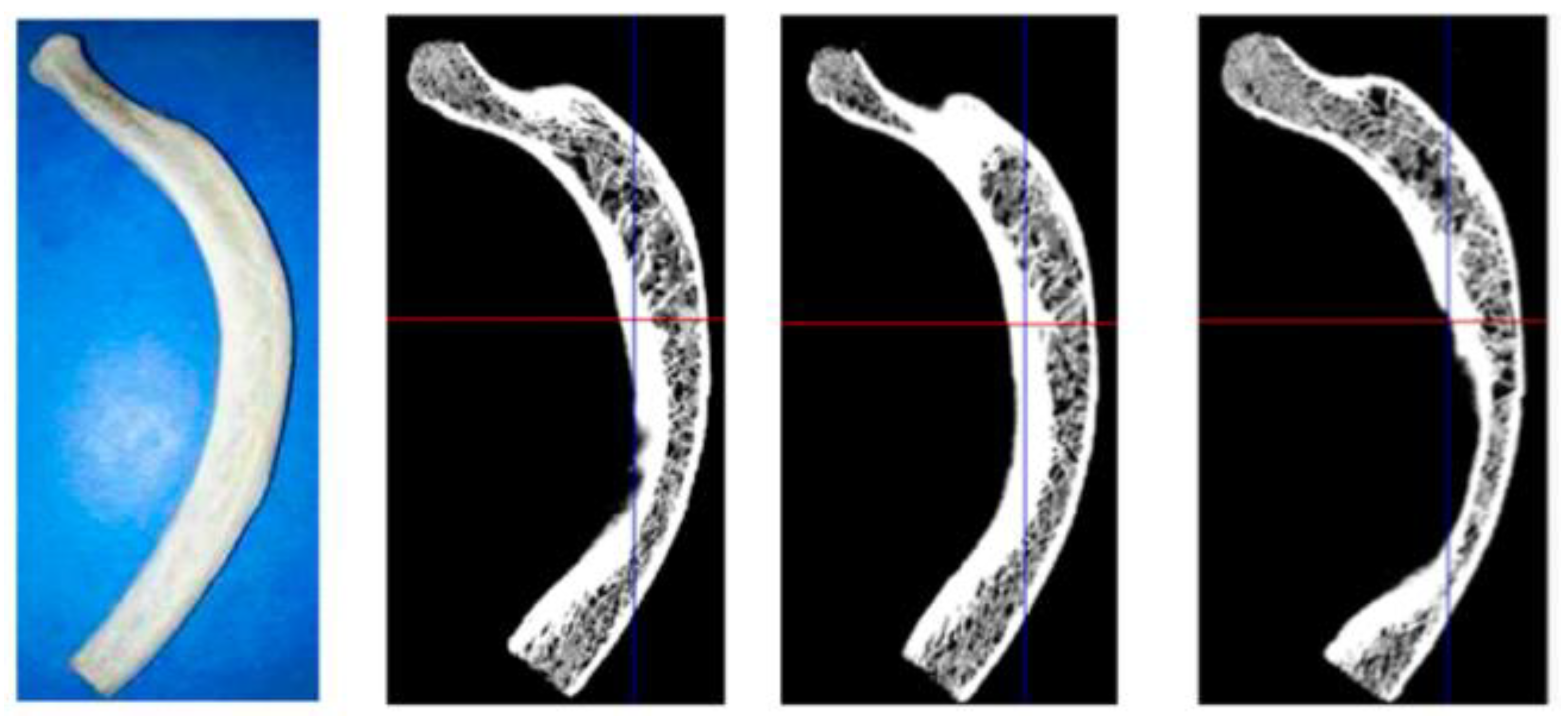
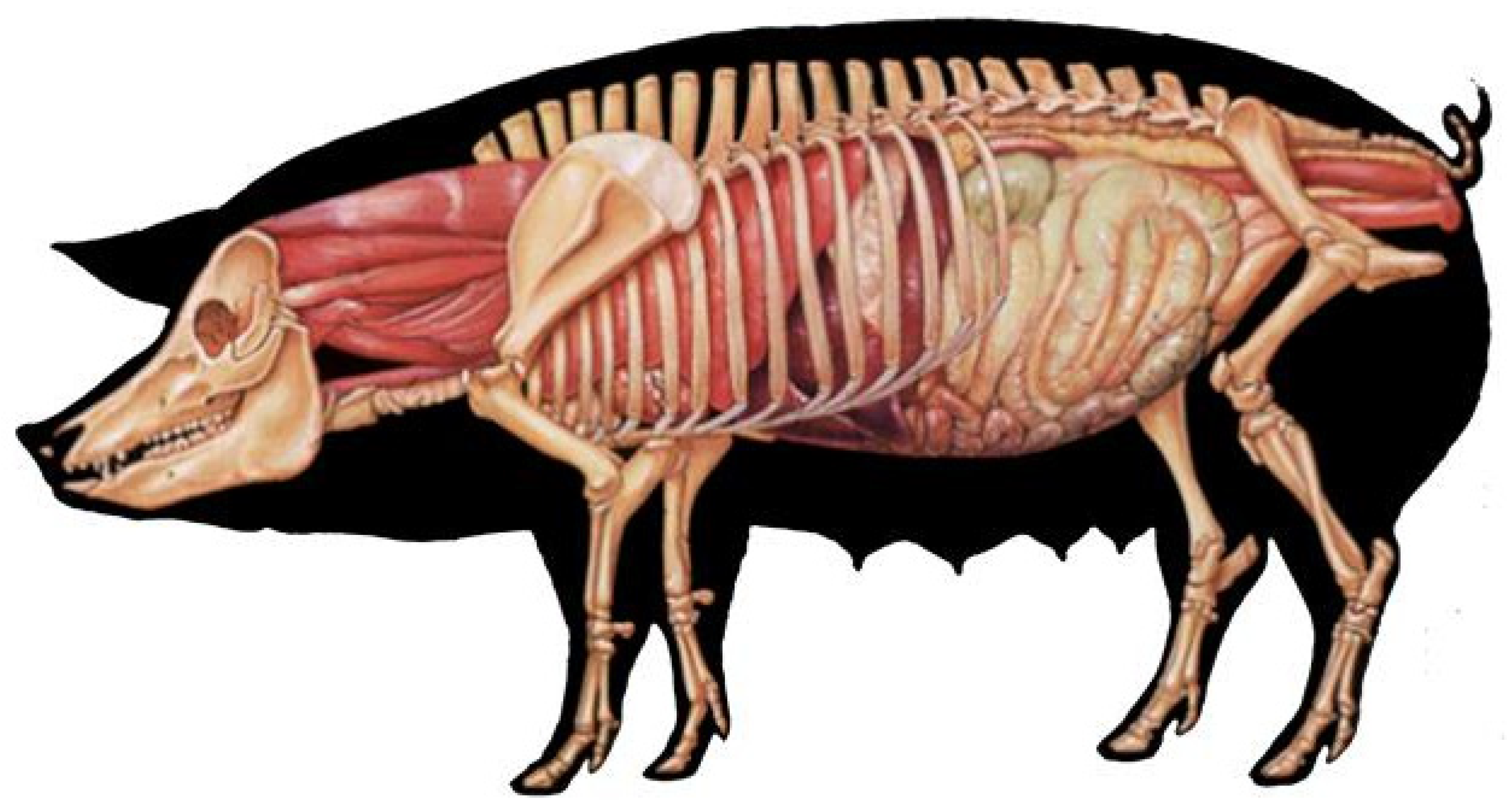
Ribs are long, arched bones that form a ring around the rib cage (Figure 3). Depending on the species, a pig’s rib cage consists of 13–17 pairs of ribs (Figure 4). The last two pairs are known as free ribs, which are not connected to the sternum. In the structure of a single rib, the shaft and the two tips—anterior and posterior—are distinguished. The diameter of the bone changes with length, where the anterior end is much thicker. This phenomenon is the result of more bone tissue, which provides a stronger connection between the ribs and the rest of the rib cage [13].

The rib shaft is the main part of the bone, which is a long and curved structure. It consists of a dense bone tissue, which provides it with strength and protection for the organs in the rib cage. It has two rib processes on the sides facing backward. The rib processes are shaped like hooks that connect to the spinous processes of the spinal vertebrae, which hold the ribs in place. The back of the rib connects to the spine through the rib–vertebral joint, which allows for a mobile connection to the corresponding vertebra of the spine. This connection provides flexibility and allows the chest to move during breathing. The front ends of the ribs connect to the sternum, which is a flat, horizontal bone located at the front of the rib cage, using rib cartilage. This is a flexible connection that allows some degree of rib movement and cushions forces during breathing. Encasing the ribs are the rib muscles, which are crucial for facilitating the movement of the rib cage during breathing. These muscles help raise and lower the ribs, allowing the space inside the rib cage to expand and contract [13].

The structure of a single rib consists of two primary layers: an outer compact layer and an inner spongy layer. The compact part, also called the cortical substance of the bone, accounts for most of the mass and volume of the bone. It mainly consists of compact bone tissue, which is a densely packed, hard, and durable form of bone tissue. It surrounds the inner spongy substance of the bone and is mainly found in the middle part of the bone. It is a porous, plexiform structure, which makes bones lighter but maintains their strength. This structure allows the body to maintain mobility while reducing stress on the body.

Table 1. Mechanical parameters of the pig’s cortical bone material [14].

Parameter	Value	Unit
Density ρ	1691.0	kg/m3
Young’s modulus E	9.38	GPa
Poisson’s ratio ν	0.3	-
Yield strength RE	70.88	MPa
Exponent of consolidation n	1.2	-

and

Table 2. Mechanical parameters of the pig’s spongy bone material [14].

Parameter	Value	Unit
Density ρ	773.0	kg/m3
Young’s modulus E	1.8	GPa
Poisson’s ratio ν	0.45	-
Yield strength RE	20.48	MPa
Exponent of consolidation n	2.0	-

show the selected mechanical properties of a cortical and spongy bone structure.

2.3. Pig’s Skin

The pig’s skin is an external, durable, and flexible organ that covers almost its entire body. It is a heterogeneous material composed of three primary layers: the epidermis, dermis, and subcutaneous tissue (Figure 5). The epidermis, the outermost layer, is primarily composed of dead cells, with a thickness ranging from 30 to 140 μm [16]. The dermis lies directly beneath the epidermis and contains collagen fibers, elastin fibers, blood vessels, sebaceous glands, and sweat glands. The innermost layer, known as subcutaneous tissue, is a fatty layer situated beneath the dermis. The average thickness of the skin in the thoracic region is 2.3 mm, and its density is 1000–1300 kg/m³, depending on the species studied [17].

From a mechanical perspective, leather is regarded as a composite material characterized by a highly hierarchical structure. Its multilayered nature also makes it a highly anisotropic material. Skin tissues exhibit viscoelastic mechanical properties, and under the action of pre-stress, it shows an uneven distribution of changes on its surface [19]. Collagen fibers play a significant role in determining the mechanical properties of the skin, particularly in their structural arrangement and orientation. The orientation of collagen fibers is not indifferent. There is a preferred orientation described as Langer lines, where there is optimal tension in the skin.

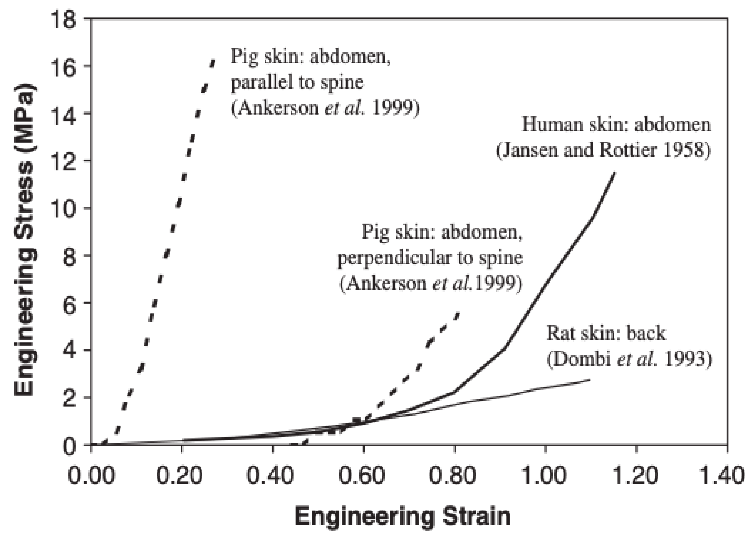
The viscoelastic properties of skin tissue are demonstrated by the hysteresis observed in the stress–strain relationship as depicted in Figure 6. The graph illustrates the energy lost within the tissue during the loading and unloading process. This phenomenon occurs as a result of internal friction, where the energy of mechanical deformation is converted to heat [20]. Skin tissue hardening under uniaxial tension begins at lower stress levels when aligned parallel to the preload direction compared to stresses transverse to the preload direction. This behavior is explained by defining skin as an orthropic material.

Determining the values of the mechanical parameters of skin tissue is challenging. Young’s modulus is estimated to range between 7.6 and 62.6 MPa, where tensile strength for samples taken parallel to the spine is 2.5–15.7 MPa [17].

3. Assumptions for Numerical Modeling

A hybrid numerical approach was used in the modeling, combining features of the finite element method (FEM) and smoothed particle hydrodynamics (SPHs). The FEM was used to simulate bodies with a homogeneous and continuous structure, characterized by a compact material structure. In contrast, the SPH method was used for materials with a discontinuous structure, such as porous materials. The porosity of these materials was only a small fraction of the total volume of the component under study, which made it impossible to accurately model the pores using the conventional FEM due to the need for a very fine discretization mesh. As a result, the two methods were combined to effectively represent the various structural properties of the materials under analysis.

Rheological models are mathematical or physical models that describe the behavior of materials under stress and strain. Nonlinear rheological models are a type of these models that account for nonlinear stress–strain relationships in a material. In studies of the properties of soft tissues such as the liver, simplified models such as the linear-elastic model are often used to describe their behavior. The linear-elastic model is versatile and allows for the analysis of a material’s behavior under different types of loading. However, this general idea has some limitations due to the assumption of a linear rheological response of the material, which can lead to errors.

In contrast, another approach describes hyper-stress models as dominant when related to viscosity. Basic diagrams of the most commonly used viscoelastic models in the mathematical description of liver tissue and the strain energy density functions of hyperelastic models are presented in

Table 3. Deformation energy density functions of models.

Model	Equation
Neo-Hooke	$W=C_1(I_1-3)$
Mooney-Rivlin	$W=\sum C_{ij}{(I_1-3)}^i{(I_2-3)}^j$
Ogden	$W=\sum \left({\displaystyle \frac{{\mu }_k}{{\alpha }_k}}\right)({\lambda }_1^{\alpha k}+{\lambda }_2^{\alpha k}+{\lambda }_3^{\alpha k}-3)$
Yeoh	$W=\sum C_k{\left(I_1–3\right)}^k$
Arruda-Boyce	$W=nkB\theta \left[{\displaystyle \frac{1}{2}}\right(I_1-3)+({\displaystyle \frac{1}{20N}}\left)\right(I_1^2-9)+({\displaystyle \frac{11}{1050N^2}}\left)\right(I_1^3-27)+\dots ]$
Veronda-Westmann	$W=C_1(e^{C_3(I_1-3)}-1)+C_2(I_2-3)$

.

Among the hyperelastic models presented in Table 3, except for the last one, all models represent polynomial functions, describing rubber-like materials subjected to large deformations. The Veronda–Westmann model, on the other hand, is an exponential model.

In order to reduce the likelihood of erroneous analysis results, a different approach is used to study the structure of the tissues. It involves describing their properties using hyperelastic and hyperelastic models [24]. These models enable more precise predictions of the mechanical behavior of various elastomers or soft tissues. Given the complexity of rheological models and the extensive input data required, the focus was narrowed to two hyperelastic rheological models: the Yeoh model and the Ogden model. Both models are widely referenced in the literature for accurately characterizing the mechanical response of the liver. A mathematical approach was selected to compare these models, emphasizing simplicity in calculations while still providing valuable data for simulations.

Yeoh’s hyperelastic material model provides a phenomenological representation of the deformation behavior of nearly incompressible and nonlinear elastic materials, such as rubber. This model builds on Ronald Rivlin’s observation that the elastic properties of rubber can be characterized using the strain energy density function, which is expressed as a power series of strain invariants.

Yeoh’s model, often referred to as the reduced polynomial model due to its polynomial format of the strain energy density function, was originally proposed in a cubic form. This formulation considers only the first strain invariant I₁ and is specifically designed for completely incompressible materials. The strain energy density function for Yeoh’s model is expressed as follows:

$$W=\sum C_k({I_1-3)}^k$$

(1)

where $C_k$ is the material’s constants (

Table 4. Yeoh model’s material constants.

Sample	Material Constants
	C10	C20	C30
1	1.414	51.352	189.630
2	1.571	36.782	452.368
3	0.418	89.325	−8.329
4	0.952	25.984	5.219

). The quantity $2C_1$ can be interpreted as the initial shear modulus.

The Yeoh mathematical model is presented below.

$$U=C_{10}\left(I_1-3\right)+C_{20}{\left(I_1-3\right)}^2+C_{30}{\left(I_1-3\right)}^3+{\displaystyle \frac{1}{D_1}}({J^{el}-1)}^2+{\displaystyle \frac{1}{D_2}}({J^{el}-1)}^4+{\displaystyle \frac{1}{D_3}}({J^{el}-1)}^6$$

(2)

$$I_1={\lambda }_1^2+{\lambda }_2^2+{\lambda }_3^2,{\mu }_0=2C_{10},K_0={\displaystyle \frac{2}{D_1}}$$

(3)

The Ogden material model is a hyperelastic framework designed to characterize the nonlinear stress–strain behavior of complex materials, including polymers and biological tissues. This model was developed by Raymond Ogden in 1972 and has since become a widely used approach for modeling the mechanical properties of such materials. The model plays a key role in determining stress–strain relationships in hyperelastic materials. It characterizes materials as isotropic, incompressible, and hyperelastic.

Similar to other hyperelastic models, Ogden’s model assumes that a material’s behavior can be characterized by a strain energy density function, which forms the basis for deriving stress–strain relationships. In Ogden’s model, the strain energy density W is expressed in terms of the principal stretches ${\lambda }_{i,j}=1,2,3.$

$$W=\sum \left({\displaystyle \frac{{\mu }_k}{{\alpha }_k}}\right)({\lambda }_1^{\alpha k}+{\lambda }_2^{\alpha k}+{\lambda }_3^{\alpha k}-3)$$

(4)

Analyzing a material that is not in compression during uniaxial stretching uses a stretching factor, defined as λ = l/l₀. Here, l represents the length after stretching, and l₀ is the original, unstretched length of the material.

$$U={\sum }_{i=1}^N{\displaystyle \frac{2{\mu }_i}{{\alpha }_i^2}}({\lambda }_1^{{\alpha }_i}+{\lambda }_2^{{\alpha }_i}+{\lambda }_3^{{\alpha }_i}-3)+{\sum }_{i=1}^N{\displaystyle \frac{1}{D_i}}({J^{el}-1)}^{2i}$$

(5)

$${\mu }_0={\sum }_{i=1}^N{\mu }_i$$

(6)

$$K_0={\displaystyle \frac{2}{D_1}}$$

(7)

For incompressible materials, the principal stresses satisfy the following condition [25]:

$${\lambda }_1{\lambda }_2{\lambda }_3=1$$

(8)

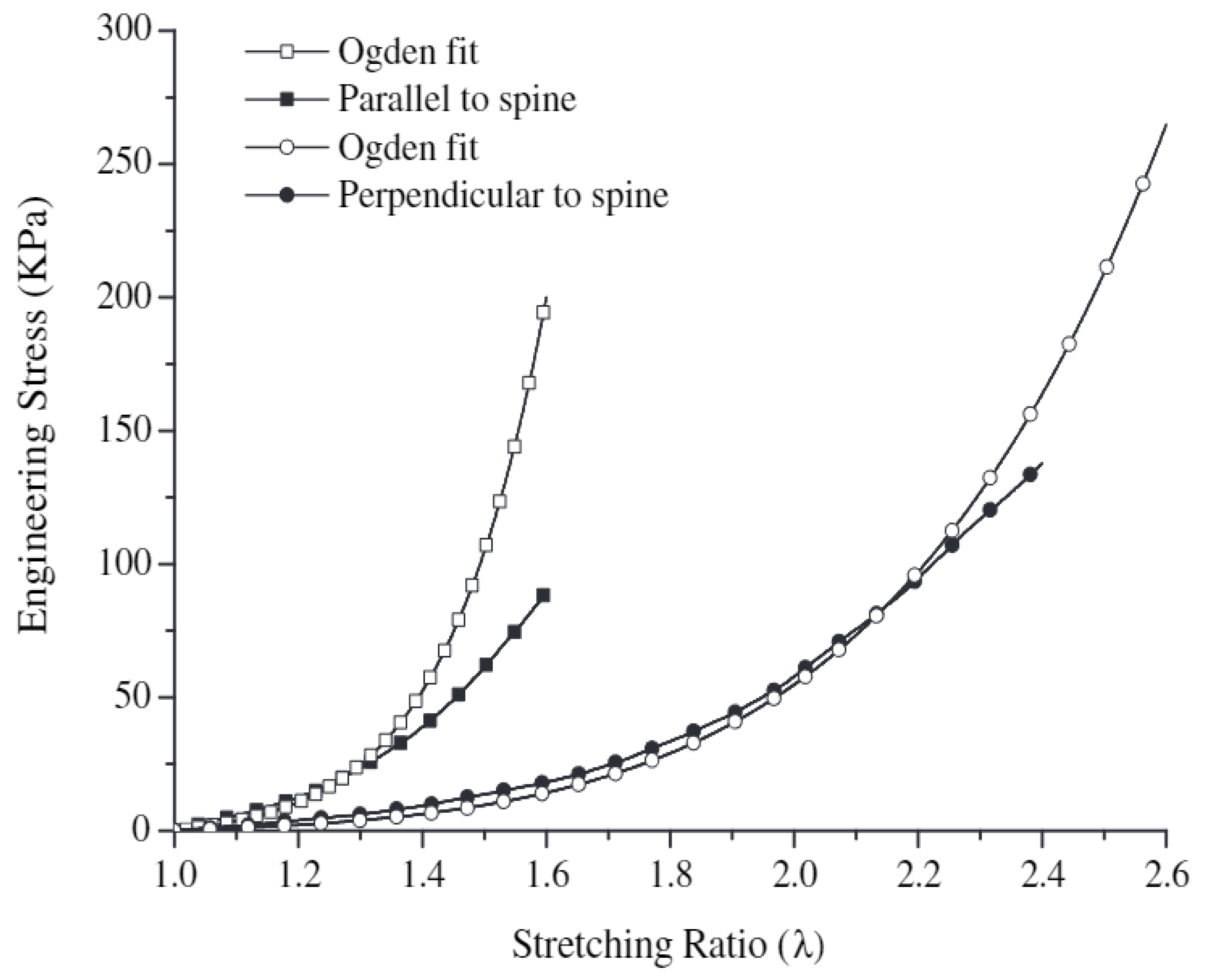
The two constants used in the Ogden model are determined through experimental data. Figure 7 shows the stress–strain curve in pig skin tension fitted to Ogden’s one-particle model in quasi-static tension. The experimentally determined Ogden constants are shown in

Table 5. Material constants of Ogden’s model.

Sample	Material Constants
	${\mathit{\mu }}_1$	${\mathit{\alpha }}_1$	${\mathit{\mu }}_2$	${\mathit{\alpha }}_2$	${\mathit{\mu }}_3$	${\mathit{\alpha }}_3$
1	0.752	53.713	127.595	1.284	41.126	5.055
2	0.242	15.052	5.452	−0.099	42.042	−0.022
3	2.220	8.878	32.485	−0.471	23.779	0.189
4	2.428	10.507	6.411	2.110	16.033	−0.782

. Having knowledge of one of the two constants in the Ogden model enables a reasonably accurate approximation of the experimental data.

Regarding the strength study of the problem under consideration, a numerical analysis was carried out using the Abaqus program. The process began with the creation of geometric models in Inventor, and then these models are exported to a computational environment in .step format. In order to describe the mechanical properties of biological materials, the Johnson–Cook rheological model was used. This is a rheological model used to characterize materials with an elastic–plastic behavior with nonlinear amplification. The initial part of the model describes the linear response of the material under a given load and is characterized by Young’s modulus and Poisson’s ratio. However, beyond this limit, the material exhibits nonlinear strengthening, which is captured by the Johnson–Cook mathematical model in a numerical analysis. The Johnson-Cook model is based on the von Mises flow stress and incorporates nonlinear strain-dependent strengthening, strain rate effects, and thermal fatigue. The Johnson–Cook model is typically expressed as follows:

$${\sigma }_y=\left(A+B{\epsilon }^{p^n}\right)\left(1+cln{\dot{\epsilon }}^{*}\right)\left(1-T^{*m}\right)$$

(9)

where

$${\dot{\epsilon }}^{*}={\displaystyle \frac{{\dot{\underset{\_}{\epsilon }}}^p}{{\dot{\epsilon }}_0}}$$

(10)

$$T^{*}={\displaystyle \frac{T-T_{room}}{T_{melt}-T_{room}}}$$

(11)

where $A$ is the yield strength of the material; $B$ is the yield strength constant; $c$ is the dynamic strengthening factor; $n$ is the strengthening exponent; $m$ is the thermal weakening factor; ${\underset{\_}{\epsilon }}^p$ is the effective plastic strain; ${\dot{\underset{\_}{\epsilon }}}^p$ is the strain rate; ${\dot{\epsilon }}^{*}$ is the dimensionless effective strain rate; ${\dot{\epsilon }}_0$ is the reference value for the strain rate; $T^{*}$ is the dimensionless (homologous) temperature; $T_{room}$ is the reference temperature; $T_{melt}$ is the melting temperature, and $T$ is the base (current) temperature.

4. Numerical Simulations and Results

Given the complexity of the rheological model and the large number of input parameters, the remainder of the paper focuses on the analysis of two specific rheological models: the Yeoh model and the Ogden model. For this purpose, preliminary numerical analyses were carried out by stimulating the process of pressing the penetrator into the liver sample. Due to the lack of available experimental results, we relied on publicly available literature data. This chapter aims to verify the numerical methods used. In order to simplify the calculations, two mathematical models that are effective for simulation applications were selected. The Ogden and Yeoh hyperelastic models, widely referenced in the literature for modeling the mechanical response of the liver, were chosen for our analysis.

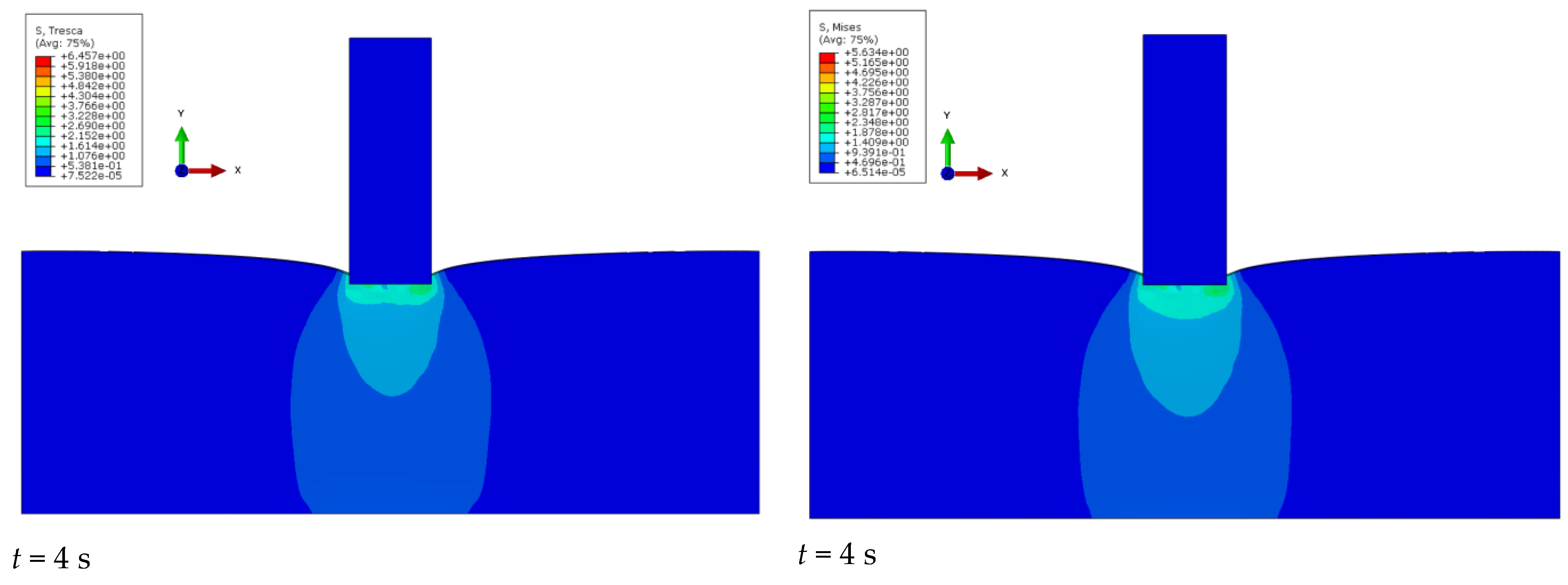
The study began by modeling the geometry of the intender and the structure of the liver. The proposed intender was cuboidal in shape with dimensions of 8 × 10 × 30 mm. In order to simplify the simulation, a cuboid of 8 × 32 × 90 mm was assumed as the liver, for which parameters were set corresponding to the mechanical properties given in the table below (

Table 6. Mechanical parameters of the pig’s liver.

Parameter	Value	Unit
Density ρ	1.075	g/cm3
Young’s modulus E	1.1	kPa
Compressive stress RC	123.0	kPa
Yield strength RE	205.0	kPa
Strain energy density	18.19	kJ/m3

).

Figure 8 shows the obtained stress results for the simulation of the intender cavity in the liver structure for four time steps. A comparison of the results obtained for the von Mises and Tresca stress results is shown.

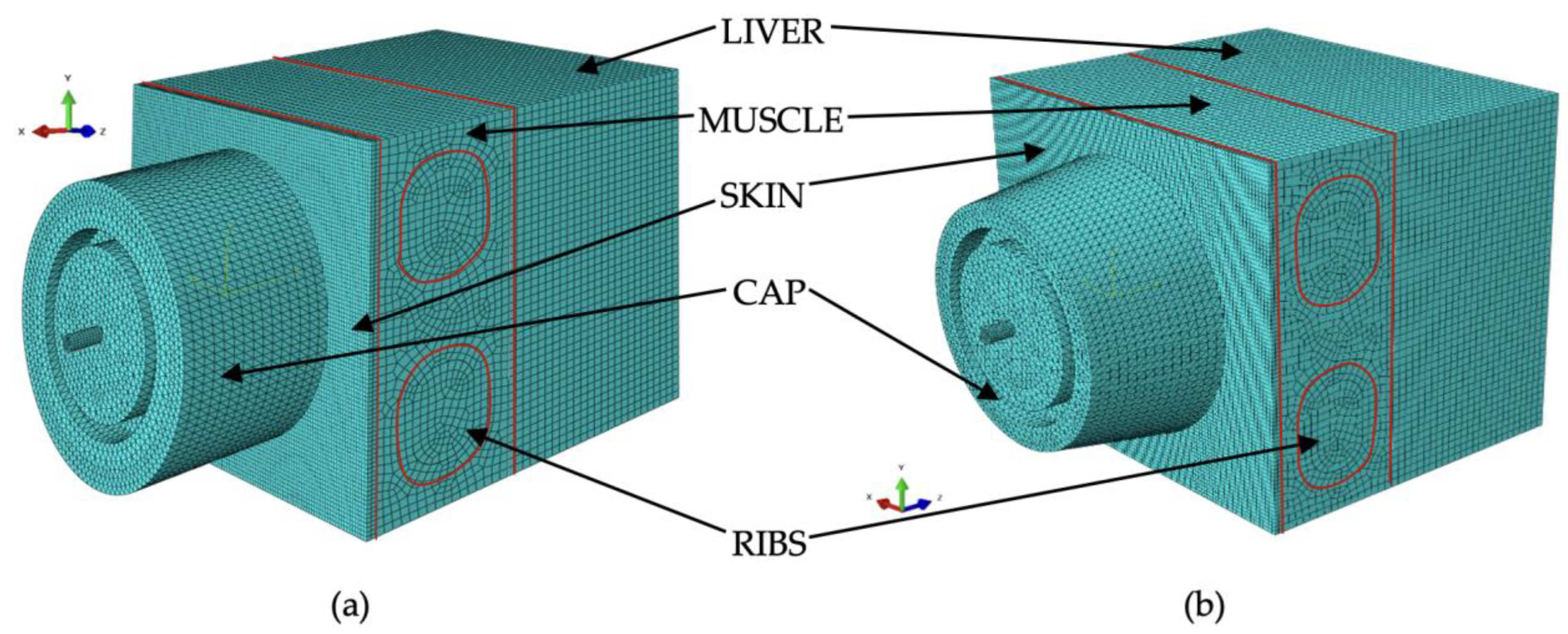
Subsequently, a numerical model of the liver structure as an organ with complex structure and geometry was developed. Then, a system was created to simulate the examination of the liver percutaneously. The process was carried out in three stages: the first focused on modeling the soft tissues, such as the skin; the second addressed the modeling of hard tissues, such as the ribs; and the third stage involved integrating the collected data with the liver model and scaling it appropriately.

In this stage, the rib component was modeled, distinguishing between the external compact layer and the internal spongy layer. The mechanical parameters required for developing the numerical models of these components are provided in

Table 7. Mechanical parameters of the cortical bone substance.

Parameter	Value	Unit
Density (ρ)	1850.0	kg/m3
Young’s modulus (E)	1.80	GPa
Poisson’s ratio (ν)	0.35	-
Johnson–Cook Model
Yield strength (A)	160.0	MPa
Fixed fortification (B)	165.0	MPa
Exponent of consolidation (n)	0.1	-

and

Table 8. Mechanical parameters of the spongy bone substance.

Parameter	Value	Unit
Density (ρ)	900.0	kg/m3
Young’s modulus (E)	18.0	MPa
Poisson’s ratio (ν)	0.4	-
Johnson–Cook Model
Yield strength (A)	42.0	MPa
Fixed fortification (B)	55.0	MPa
Exponent of consolidation (n)	0.9	-

. Due to its porous structure, the spongy part of the bone was modeled using smoothed particle hydrodynamic (SPH) elements, while the remaining parts were modeled using the finite element method (FEM).

A series of numerical simulations were performed on the developed geometric models, incorporating initial and boundary conditions, as well as parameters for simulating the liver’s loading within the elastic range. The first numerical analysis focused on a single rib. The rib’s average length ranged between 30 and 40 cm, with a typical width and depth between 5.5 and 7.5 cm, which was measured along its curved length [13]. For this study, these values were averaged across the majority of the population. The model was discretized with a resolution of 0.5 mm, employing Tetra-type elements for the simulation. The goal was to represent the wave motion that occurs when performing elastography. A rectangular-shaped inductor was used in the analysis.

In addition, numerical simulations were carried out at various signal frequencies, from 1.0 to 5.0 MHz. Based on the results, hard tissues were analyzed to evaluate the accuracy of the modeling for both cortical and spongy structures, as well as the bone’s capacity to absorb sound waves. Finally, a comprehensive model combining soft tissues, hard tissues, and liver elements was validated to ensure its accuracy and reliability.

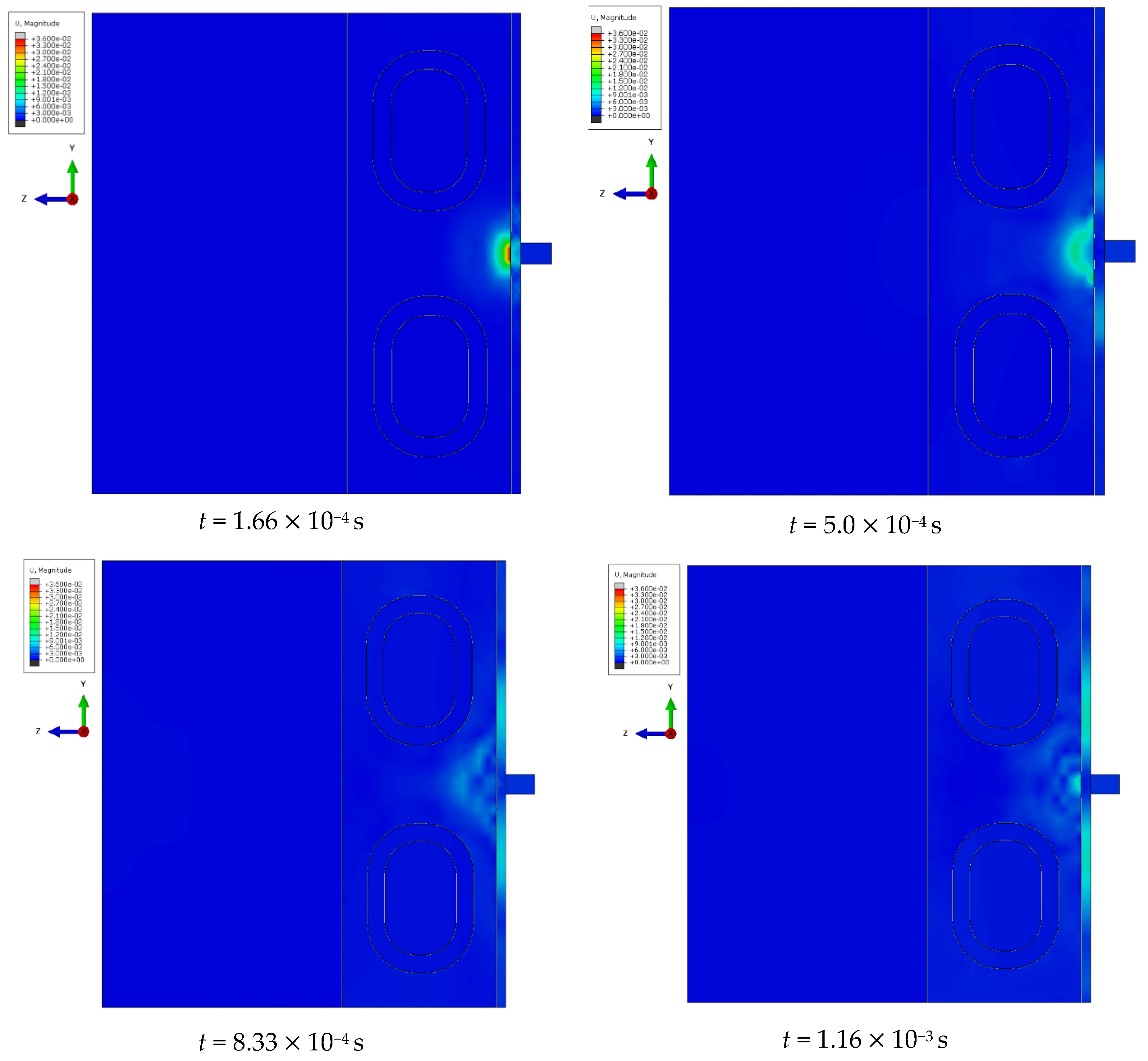
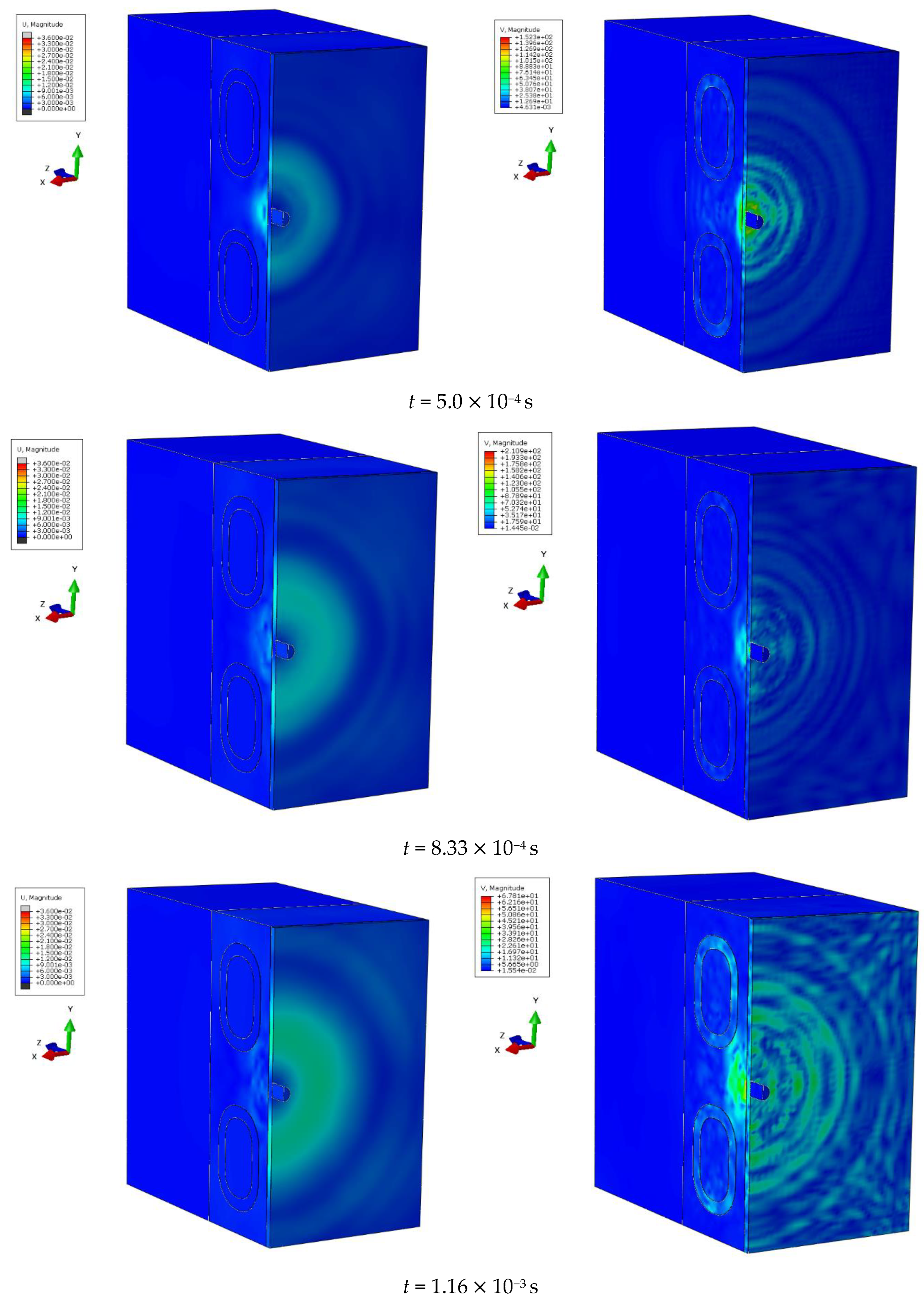
The simulation results of mechanical wave propagation through tissues, ribs, and the liver without an additional cap revealed the occurrence of interference phenomena at the level of the rib bones (Figure 9 and Figure 10). Subsequent stages of the simulation were excluded due to wave reflection at the liver’s edge, as the model did not include adjacent organs. The wave’s effects were meticulously analyzed within a frequency range of 1.0 to 5.0 MHz, liver tissue stiffness between 2.7 and 16.5 kPa, and a liver steatosis level below 270 dB/m. From this analysis, the speed of sound propagation in the studied environment was determined. Specifically, for an excitation frequency of 3.5 MHz, the simulation yielded a propagation velocity of 1420 m/s.

Tests were carried out for the use of the FibroScan^® device together with the six types of caps designed. Two geometric designs for the caps were selected for analysis: a cylindrical one using the designation E15 and a conical one referred to as D0. Tetra-type elements with an additional node inside were adopted for discretization. Geometric models were made based on technical documentation. Figure 11 shows the adopted layout with the overlays undergoing discretization.

From conducting preliminary simulations, it was noted that the size of the discretization component of the model does not affect the results obtained (

Table 9. Summary of the results for a cylindrical head with different discretization sizes.

Cap	Frequency of the Inductor [MHz]	Wave Velocity [m/s]	0.5 mm	1.0 mm	1.5 mm	2.0 mm
cylindrical	1.0	843	843	842	842	842
	1.5	906	906	905	905	906
	2.0	969	969	969	969	969
	2.5	992	991	992	991	992
	3.0	1050	1050	1051	1050	1050
	3.5	1083	1082	1082	1083	1082
	4.0	1132	1132	1132	1132	1132
	4.5	1183	1182	1182	1183	1184
	5.0	1243	1245	1244	1243	1244
Cap	Frequency of the inductor [MHz]	Wave velocity [m/s]	2.5 mm	3.0 mm	4.0 mm	5.0 mm
cylindrical	1.0	843	841	843	843	843
	1.5	906	906	905	905	906
	2.0	968	969	968	968	969
	2.5	992	991	992	991	992
	3.0	1050	1051	1050	1051	1050
	3.5	1083	1082	1083	1082	1082
	4.0	1132	1132	1132	1132	1132
	4.5	1183	1182	1182	1182	1182
	5.0	1245	1243	1244	1243	1245

). The individual variables in each frequency occur due to the way the computer software represents the results and does not affect the result (rounding of numbers).

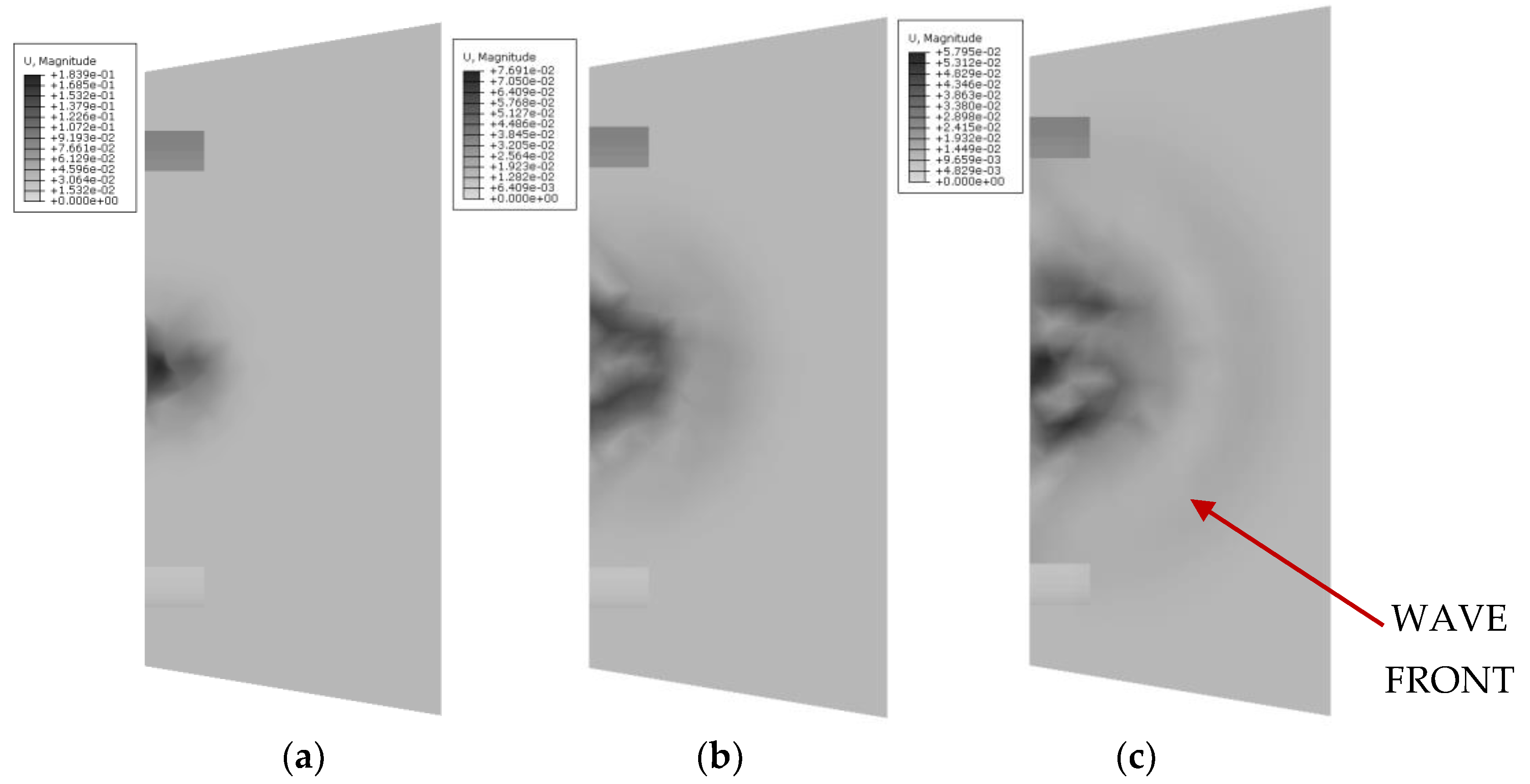
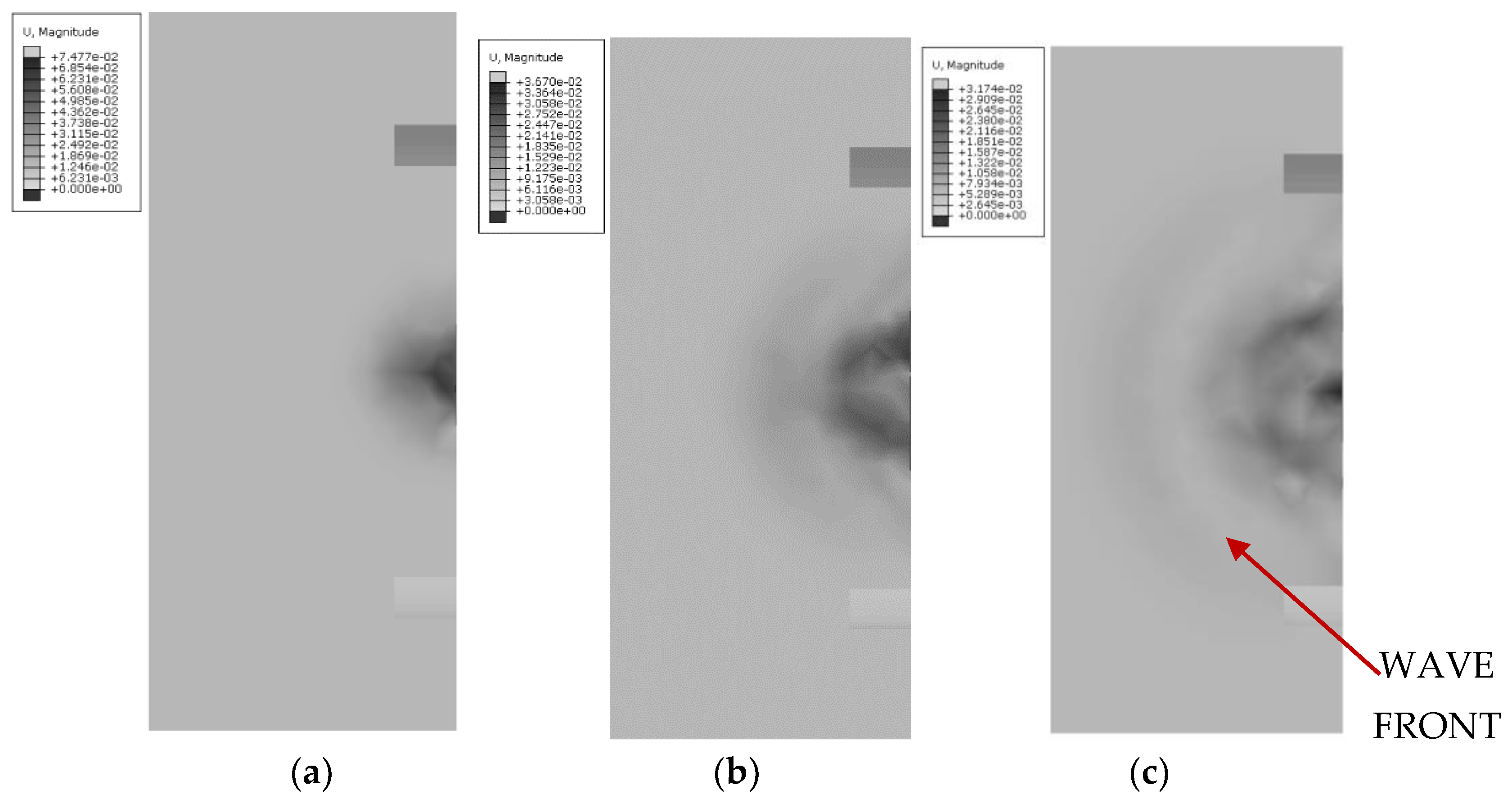
In the first stage of wavefront propagation studies, a numerical analysis was conducted on two types of cap geometries: conical and cylindrical, with an assumed wave excitation frequency of 3 MHz. Figure 12 presents a summary of wave propagation for the conical cap at successive time moments: 3.3 $\times$ 10⁻⁴ s, 6.6 $\times$ 10⁻⁴ s, and 1.0 $\times$ 10⁻³ s. The observations show how the size and intensity of the wave change as the propagation process continues through the medium.

In comparison, Figure 13 illustrates the wave propagation for the cylindrical cap at the same time moments: 3.3 $\times$ 10⁻⁴ s, 6.6 $\times$ 10⁻⁴ s, and 1.0 $\times$ 10⁻³ s. This comparison allows for an assessment of how the cap geometry influences the shape and scattering of the mechanical wave. The differences in propagation are evident in the way the wave spreads and in the efficiency of energy dispersion within the medium, which is crucial for further analysis of the models’ effectiveness.

This approach enables the evaluation of which geometry better reduces wave intensity, which is significant for applications in non-invasive medical examinations, such as liver assessment using a cap model.

Initially, the caps were made by using three different materials: Agar, Ecoflex 00-20, and Medical Gel. Based on the results obtained on experimental animals and post-mortem organs, the best-fitting material in relation to the tissue under study was selected, which turned out to be Ecoflex 00-20.

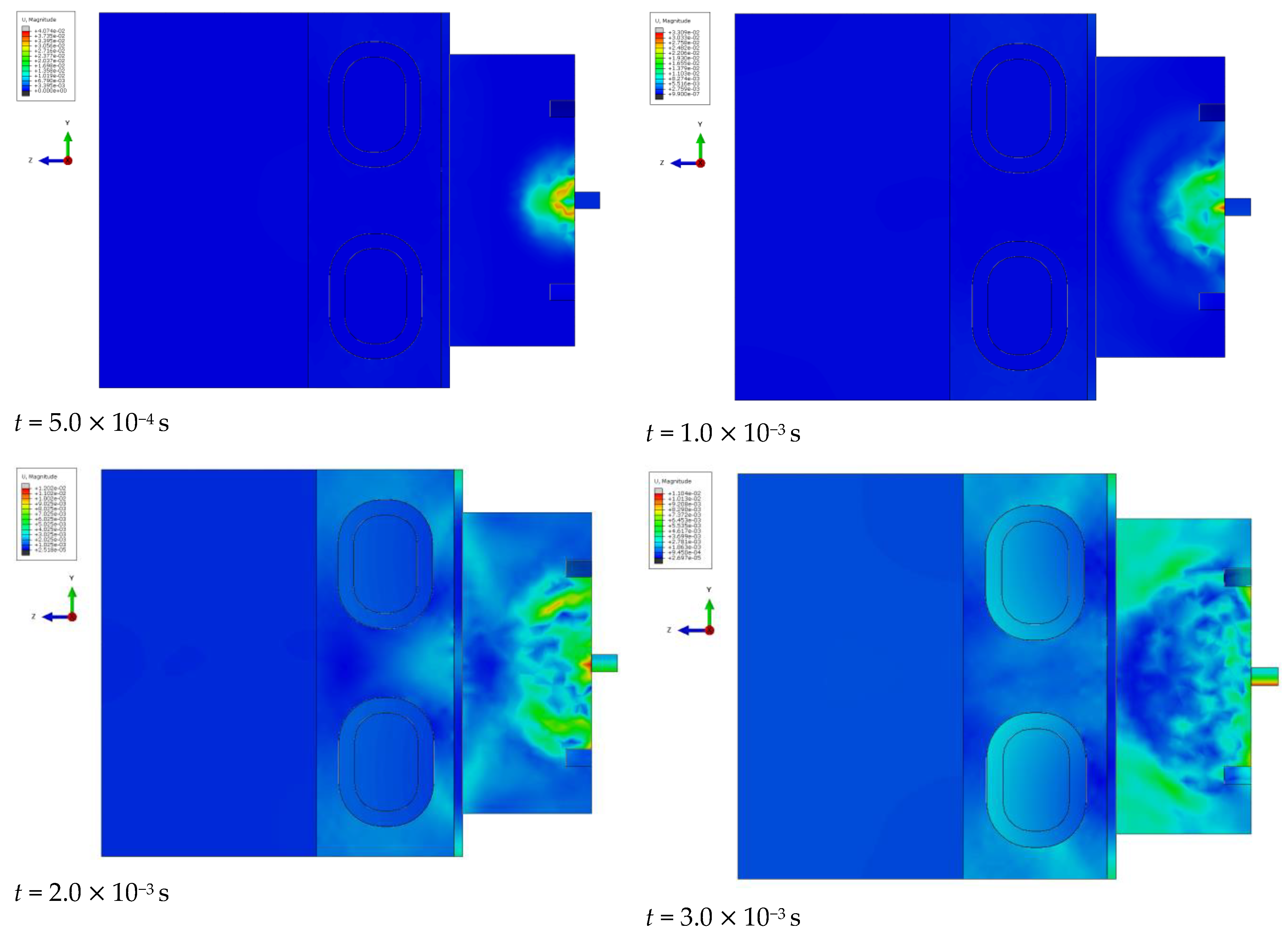
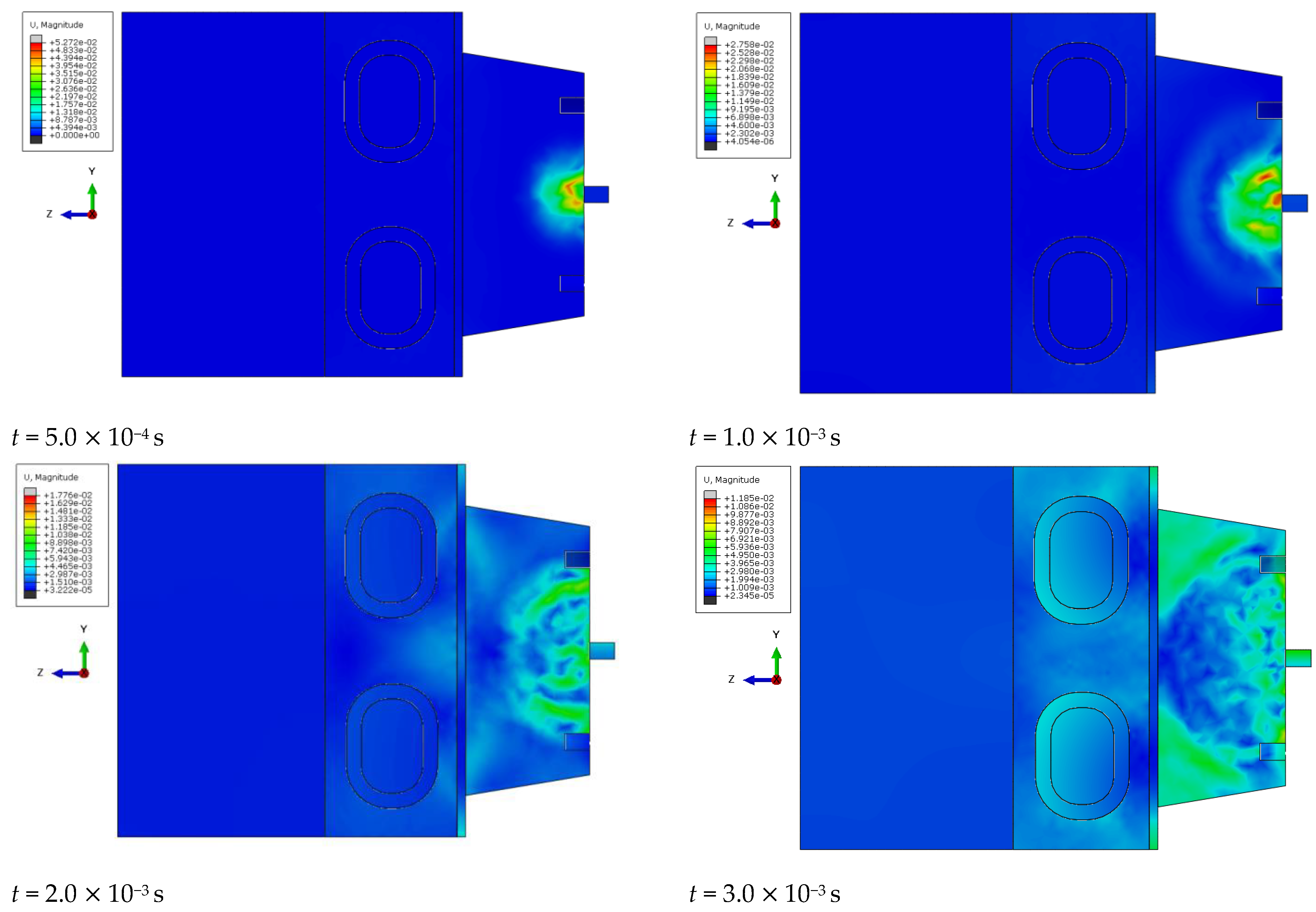
A numerical analysis was carried out while maintaining the set frequency for the inductor at 1.0–5.0 MHz. The following is an example of the results obtained for caps made of the Ecoflex 00-20 material using an exciter frequency of 2.0 MHz. The change in displacement during the phenomenon and the value of attenuation (CAP) in relation to the obtained stiffness were analyzed depending on the mathematical model used. The juxtaposition of damping results for different numerical models using a conical cap and a cylindrical cap made of the Ecoflex 00-20 material (Figure 14 and Figure 15) is important in the context of comparing their effectiveness in reducing the intensity of the mechanical wave (

Table 10. Summary of the damping results for the applied numerical models using a cylindrical cap made of the Ecoflex 00-20 material.

Mathematical Model	Name	CAP (dB/m)	E (kPA) Median
Yeoh	flank	240	4.7
J-C	breastbone	172	11.2
J-C	back	213	9.7
Yeoh	flank	242	8.2
J-C	breastbone	253	7.5
J-C	back	214	4.3
Odgen	flank	241	6.5
J-C	breastbone	223	8.9
J-C	back	165	7.1
Odgen	flank	264	13.4
J-C	breastbone	241	3.6
J-C	back	157	3.8

and

Table 11. Summary of the damping results for the numerical models using a conical cap made of the Ecoflex 00-20 material.

Mathematical Model	Name	CAP (dB/m)	E (kPA) Median
Yeoh	flank	245	5.1
J-C	breastbone	184	10.2
J-C	back	201	9.3
Yeoh	flank	256	8.5
J-C	breastbone	248	5.9
J-C	back	211	5.1
Odgen	flank	236	6.9
J-C	breastbone	213	7.8
J-C	back	185	8.3
Odgen	flank	281	15.4
J-C	breastbone	223	4.3
J-C	back	157	4.9

).

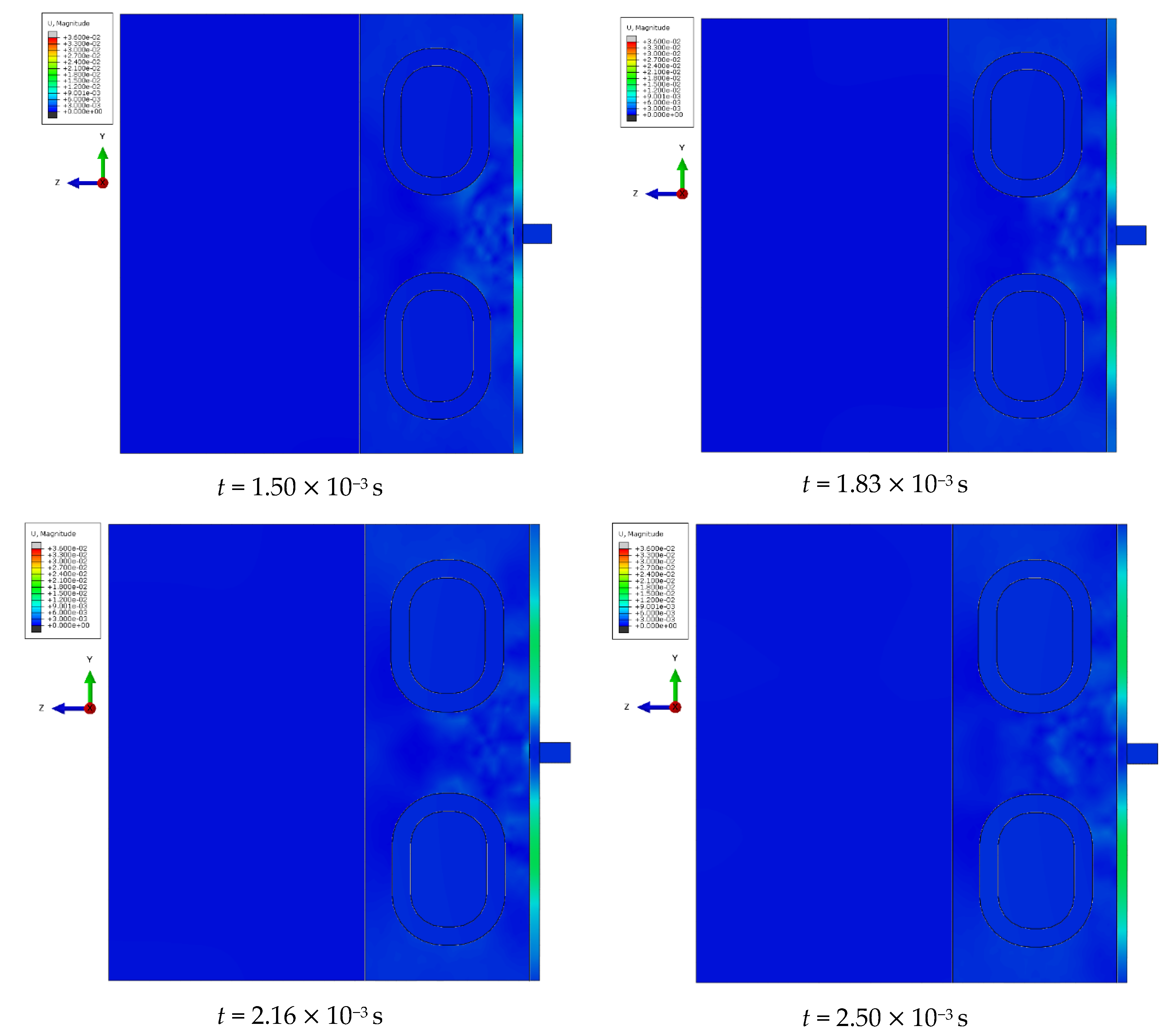
At specific time steps, i.e., t = 5.0 $\times$ 10⁻⁴ s, t = 1.0 $\times$ 10⁻³ s, t = 2.0 $\times$ 10⁻³ s, and t = 3.0 $\times$ 10⁻³ s, changes in the displacements of the wavefront within the simulated liver tissue can be observed. These displacement values indicate the evolution of the mechanical wave within the tissue under study. At the initial time step, t = 5.0 $\times$ 10⁻⁴ s, the wave is in its early propagation phase, traveling along the cylindrical applicator and progressing through the tissue as a longitudinal wave. As time progresses, i.e., at subsequent time steps, the wave gradually spreads through the simulated tissue, moving further from the generating source. By the final time step, in the description of the mechanical wave, the wavefront extends to a greater distance from the cylindrical applicator. A portion of the wave is absorbed by the bony structures present in the system, such as the ribs.

The cylindrical design of the applicator directly impacts the mechanics of wave propagation within the tissue. The shape of the tool affects the wave properties, including its amplitude, and plays a significant role in its interaction with the examined tissue during the simulation of a percutaneous liver assessment.

The conical applicator represents a geometric form that influences the focusing or scattering of the wave within the examined tissue. At the first time step, t = 5.0 $\times$ 10⁻⁴ s, an early stage of wave propagation from the conical applicator is observed. The area where the wave is noticeable is limited and does not extend to greater distances, similar to the early stage described in the previous phenomenon. As time advances, at subsequent time steps, the conical shape of the applicator enables the observation of wave dispersion within the studied medium. By the final time step, t = 3.0 $\times$ 10⁻³ s, the area in which the wave is observed reaches its maximum size, but the intensity is significantly diminished. The wavefront displacement values also change over time. At the first time step, the displacement reaches a maximum value of 0.05 mm, while at the final time step, it decreases to 0.01 mm, corresponding to the described decrease in wave intensity as it propagates through the simulated medium.

In conclusion, the shape of the conical applicator has a crucial impact on wave propagation in the tissue during the simulation of a percutaneous liver assessment. This tool shape determines the area and intensity of the wave as well as its behavior in the examined tissue at the different time stages of the simulation.

5. Validation Research

FibroScan^® technology represents a leading technique for assessing liver stiffness. This technique utilizes a low-frequency acoustic wave to non-invasively measure the stiffness of liver tissue. One of the key parameters characterizing this technology is tissue elasticity, denoted by the elasticity parameter E. In this study, applicators with two geometric shapes were considered: a cylindrical shape, designated as E15, and a conical shape, referred to as D0, both constructed from the Ecoflex 00-20 material.

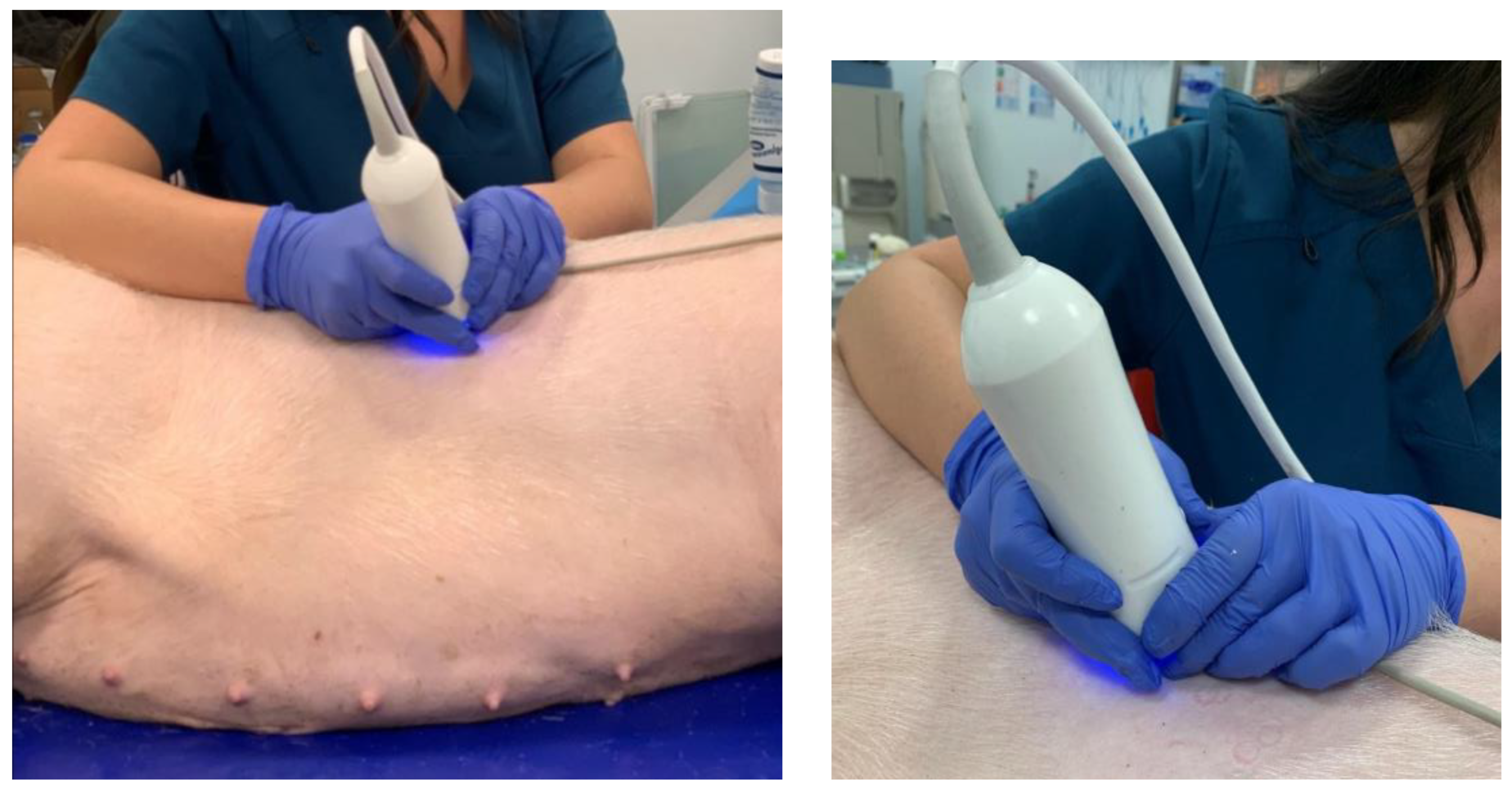
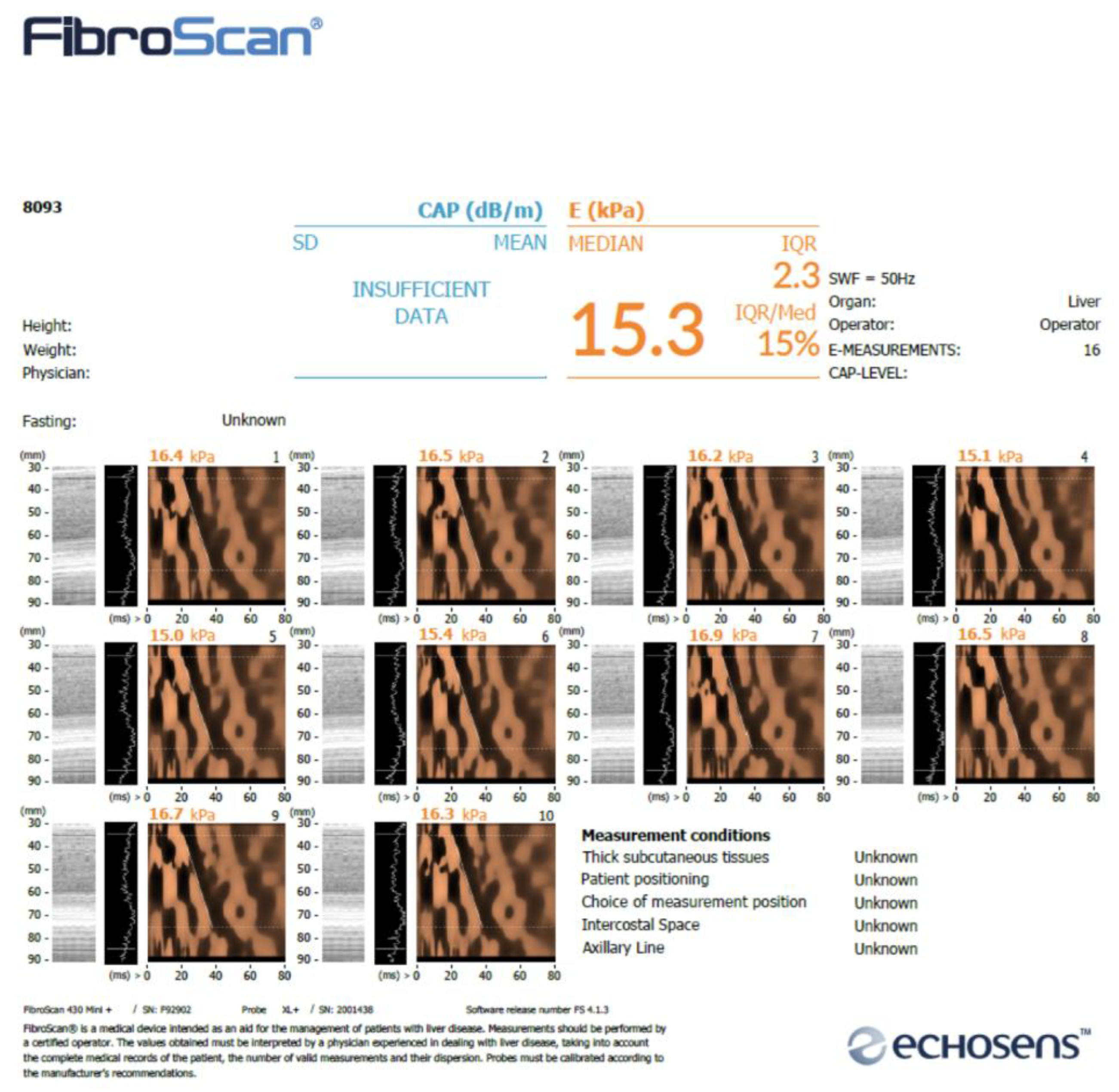
Validation studies of liver stiffness measurements were conducted using the FibroScan^® device in percutaneous assessments (Figure 16), taking into account the elasticity parameter E, which was expressed in kPa [27]. Advanced numerical models of liver tissues were developed and utilized to perform numerical simulations in the Abaqus software, allowing for the evaluation of the accuracy and effectiveness of this technology under various clinical conditions.

To conduct a comparative analysis of the results obtained from numerical simulations against reference data derived from histological studies and in vivo measurements on pigs using the FibroScan^® (Figure 17), the outcomes for the Ecoflex material are presented in

Table 12. Summary of the results for validation.

Research on Organs				Numerical Simulations
Pig no.	Date	Cap	E (kPA) Median	Cap	E (kPA) Median
W8 8236	9 March 2023	Ecoflex D0	17.4	Ecoflex D0	11.1
		Ecoflex E15	19.0
W7 8337	9 March 2023	Ecoflex D0	11.4	Ecoflex D0	6.5
		Ecoflex E15	7.7
W6 8252	9 March 2023	Ecoflex D0	24.7	Ecoflex D0	17.6
		Ecoflex E15	23.5
W5 8093	9 March 2023	Ecoflex D0	15.2	Ecoflex D0	18.2
		Ecoflex E15	15.3
W2 0590	22 December 2022	Ecoflex D0	14.2	Ecoflex E15	7.5
		Ecoflex E15	-
W1 0586	22 December 2022	Ecoflex D0	12.7	Ecoflex E15	16.6
		Ecoflex E15	-
W3 0630	22 December 2022	Ecoflex D0	16.5	Ecoflex E15	10.2
		Ecoflex E15	-
W4 0661	22 December 2022	Ecoflex D0	19.5	Ecoflex E15	13.4
		Ecoflex E15	-

.

The study involved eight Polish landrace pigs sourced from the same breeding facility. Female pigs aged 16–20 weeks with an initial weight of 40–45 kg were selected for the experiments. Elastographic measurements were conducted four times at weekly intervals. Prior to the study, all animals were acclimatized to the handling and grooming procedures. The pigs were fed an identical full-portion feed mixture in accordance with nutritional standards and kept under uniform husbandry conditions. Animal care was conducted in compliance with the National Institutes of Health guidelines for the care and use of laboratory animals. The experiments were approved and carried out in accordance with the regulations set forth by the Local Ethics Committee in Wrocław (Approval No. 46/2022/P1 dated 16 November 2022).

Elastographic examinations were conducted under general anesthesia using propofol (2 mg/kg) and isoflurane (1.5 vol%), following premedication with ketamine (10 mg/kg), midazolam (0.3 mg/kg), and medetomidine (0.03 mg/kg), with the animal positioned on its left side. An example result of liver elasticity measurement in a pig was obtained using the FibroScan^® Mini + 430 device equipped with an XL probe (5 MHz) and a stabilization-enhanced applicator, and the liver was placed in a specialized container.

No significant correlation was demonstrated between liver elasticity, measured directly in liver samples (Elasto direct; E kPa), and the results were related to non-invasive liver steatosis and liver elasticity obtained from in vivo animal studies (

Table 13. Pearson correlation coefficients calculated for 8 animals.

Variable	Mean	Std. Deviation	Correlation Coefficient
			Elasto Direct E (kPa)	CAP (dB/m)	SD	E (kPA) Median	IQR/Med.
Elasto direct E (kPa)	16.7	5.6	1.000	−0.283	−0.061	−0.258	−0.267
CAP (dB/m)	52.8	11.9	−0.283	1.000	0.174	0.214	0.288
SD	17.9	1.2	−0.061	0.174	1.000	0.407	0.689
E (kPA) median	10.0	3.8	−0.258	0.214	0.407	1.000	0.032
IQR/Med.	0.4	0.2	−0.267	0.288	0.689	0.032	1.000

). The liver elasticity results (direct) were analyzed using a one-way analysis of variance (ANOVA). The application of the FibroScan^® device probe in liver stiffness measurement was considered, with the elasticity parameter E expressed in kPa.

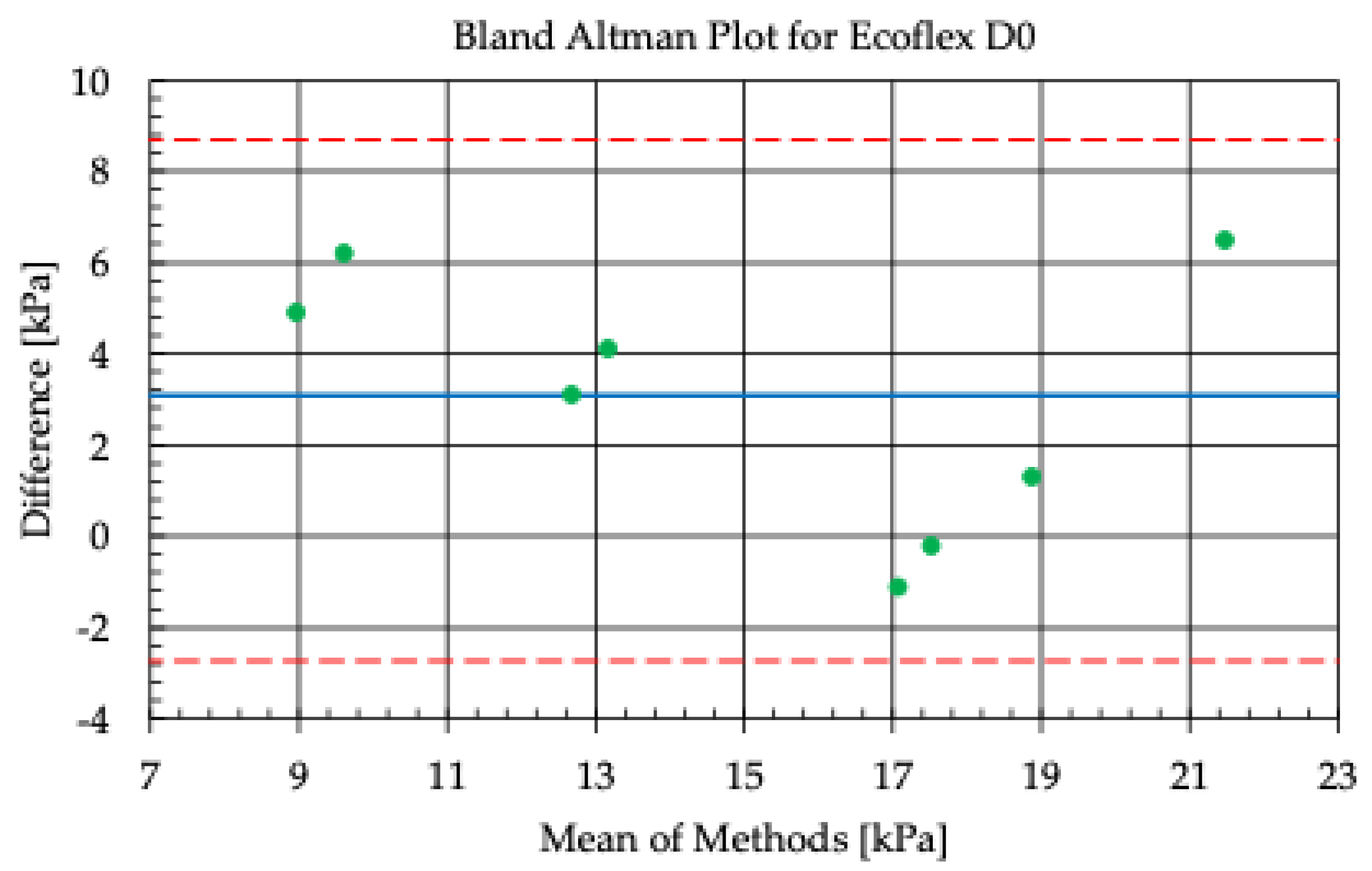
Figure 18 and Figure 19 show the results of the analysis of the agreement of elasticity measurements in kPa, obtained using the FibroScan^® applicator with a conical overlay (D0) and a cylindrical overlay (E15) made of the Ecoflex 00-20 material. The horizontal axis of the graph (x) shows the average elasticity values determined using the direct and simulation methods, while the vertical axis (y) represents the differences between these values for each measurement.

The graph shows the middle line (blue), which represents the average difference (bias) between the results of the two methods, as well as the dashed lines (red) marking the limits of agreement (limits of agreement), calculated as ±1.96 standard deviations from the average difference. Most of the points on the graph are within the limits of agreement, indicating good agreement between the direct and simulation methods.

The variation in results may be due to differences in the geometry of the applicator, the properties of the Ecoflex 00-20 material, and local differences in the mechanical properties of the tissue being tested. The limits of agreement show the range within which the differences between the methods are statistically acceptable, confirming that the measurement and simulation method used is consistent in analyzing the elasticity of the tissue under the specified conditions.

6. Results and Discussion

Numerical analysis results indicate that no significant differences were observed in the outcomes associated with the applied mathematical model. Both the Yeoh and Ogden rheological models produced comparable results, with the differences being negligible. The variance in the results, approximately 8%, represents a very good fit. Greater discrepancies were noted in the constant parameters used in the calculations—the obtained results upon altering these parameters showed larger variations within ±27%. Nevertheless, these results were deemed satisfactory, likely due to significant variability in the initial data of the rheological models. These results were used in further numerical simulations.

In the frequency range of 1.0–5.0 MHz, ultrasound attenuation in the skin increases with frequency, averaging from several to over ten dB/cm. Excessive attenuation within the scanning device’s applicator could weaken the ultrasonic wave entering the liver tissue, leading to measurement errors or making measurements impossible. The analysis employed durable gel-like or rubber-like materials with attenuation in the range of several to over ten dB/cm, which enabled accurate results.

The results of the conducted studies indicate that the shear wave velocity increases with increasing tissue stiffness, which is confirmed in the literature [6]. However, it should be noted that higher stiffness does not necessarily mean higher wave frequency, which may be a limitation due to the characteristics of the device and its configuration according to the manufacturer’s recommendations. This limitation may affect the interpretation of results under other test conditions. Future studies should consider the possibility of using other device configurations or alternative measurement techniques to compare results.

All elastography studies conducted on experimental animals using the percutaneous technique yielded valid results. In experiments performed on livers collected immediately post-euthanasia, measurements were successfully obtained using all applicator types on four livers placed in a specially prepared container that simulated the shape of a human liver. In the first four cases, where the livers were placed in a standard organ retrieval dish, measurements could not be obtained. Additionally, the first batch of agar-based applicators was prone to damage, preventing measurements, but this issue did not occur with applicators made of Ecoflex 00-20.

Using the Johnson–Cook rheological model resulted in an excellent fit for both the compact and spongy bone structures, such as the ribs. Moreover, applying the hybrid FEM/SPH method in this case yielded very satisfactory results. The spongy bone structure proved to be an excellent model for SPH applications.

The presented numerical analysis results for the preliminary assessment of the effectiveness of mechanical wave propagation, following the application of the scanning device to the examined organ, confirm the correctness of the adopted methodology. The wave velocity result (1420 m/s) correlates well with the healthy liver value (1480 m/s), indicating a very good match.

A comparative analysis between Table 10 and Table 11 highlights the differences in attenuation results for various numerical models using two types of Ecoflex 00-20 applicators. For the Yeoh model, in the case of the cylindrical applicator, the attenuation values (CAP) for the side are 240 and 242 dB/m, while for the conical applicator, they are 245 and 256 dB/m. It is noted that the attenuation values are similar for both applicators, but slightly higher for the conical one. For the Johnson–Cook model in different configurations (bridge, back) for cylindrical and conical applicators, the attenuation differences are more varied. Generally, the attenuation results for the cylindrical and conical applicators in this model do not show a consistent pattern—some cases yield similar values, while others differ more. For the Ogden model, side attenuation results for the cylindrical applicator are 241 and 264 dB/m, and for the conical applicator, the values are 236 and 281 dB/m. Attenuation values for this model show some differences between applicators, with the conical applicator sometimes reaching higher values. In summary, the attenuation analysis results for the different numerical models using cylindrical and conical Ecoflex 00-20 applicators show no clear rule for which applicator yields better attenuation results across all models. Attenuation values differ between applicators for different models, indicating the complexity of the applicator geometry’s impact on attenuation properties in numerical studies.

Chapter 5 validates the numerical simulation results by comparing them with data from report number N0CBR000.7117.SS.30/Wet/2022 [27]. Liver elasticity measurements with the E15 applicator hover around similar values, regardless of the measurement method (porcine liver measurements or numerical simulations). The average liver elasticity with the E15 applicator (numerical simulations) was 11.6 kPa. Conversely, liver elasticity measurements with the D0 applicator showed variability, both in porcine liver measurements and numerical simulations. The average liver elasticity with the D0 applicator (numerical simulations) was 15.2 kPa. It is noted that the applicator shape significantly affects liver elasticity measurement results. The conical applicator (D0) tends to yield higher liver elasticity values compared to the cylindrical applicator (E15), both for direct organ measurements and numerical simulations. These differences may be due to varying mechanical properties and the interaction of the applicator shapes with liver tissue, as well as their influence on sound wave transmission during measurements.

This study verified applicator geometries using numerical models on animals within the measurement frequency range of 1.0–5.0 MHz, covering the following parameters: liver fibrosis between 1.5 and 12.5 kPa and steatosis < 5%, 5–33%, 33–66%, and above 66%. The numerical simulation results were referenced against a healthy liver baseline value, with liver stiffness at 4.5 kPa and steatosis below 300 dB/m. Experimental and simulation results correlate, confirming the validity of the study.

7. Patents

Elastograph head cap insert, elastography measurement kit, and kit application. PCT application number: PCT/PL2023/050100 from 30 November 2023. Tiba Sp. z o.o., Wroclaw, Poland.