Improving Condensation Modelling in RELAP5: From Code Modification to Uncertainty Analysis of HERO-2 Experimental Data

Abstract

In recent decades, international interest has grown in the design and implementation of evolutionary reactors based on passive systems. The design of such systems requires reliable and validated numerical tools capable of simulating phenomena driven by very small forces, especially when compared to active systems. For this reason, several international research projects aim to assess the capabilities and limitations of numerical tools in modelling passive systems and their associated physical phenomena. The HERO-2 facility was designed to provide preliminary experimental data for characterizing bayonet tubes and exploring their potential application as Steam Generators (SGs) in advanced nuclear reactor designs, such as Small Modular Reactors (SMRs). Following the agreement between the Italian Ministry of Economic Development and the ENEA, multiple experimental campaigns were conducted, and a RELAP5 (R5) input deck of the facility has been developed. Considering the RELAP5 limits in simulating condensation phenomena encountered in previous studies, the primary objective of this study is to enhance the capabilities of the code in simulating condensation phenomena in horizontal pipes under natural circulation conditions with the implementation of Thome correlation and, in the second instance, to re-evaluate the numerical model of the HERO-2 facility. Moreover, a comprehensive uncertainty analysis (UA) is carried out to identify the key parameters influencing the simulations. The analysis revealed that the simulation results are strongly affected by the filling ratio uncertainties, a given initial condition that, together with the power supplied, determines the most important thermal-hydraulic (T/H) test parameters, such as the saturation pressure, the void fraction, mass flow rate, etc. Overall, the study provides a deeper understanding of the factors governing passive system performance and highlights the importance of accurately characterizing the experimental boundary and initial conditions in the verification and validation activities of a T/H code.

1. Introduction

The safety of Nuclear Power Plants (NPPs) is fundamental for the development of nuclear technology. Its acceptance relies on the increase in safety in order to minimize or eliminate the possible radiological risks; therefore, the strengthening and increased strictness of the nuclear safety regulation included a solid safety assessment also considering accident simulations.

Over the last decades, the interest around the passive safety systems topic has increased, considering them as one potential solution to achieve the required safety and economic requirements. However, phenomena such as natural circulation rely on weak driving forces, such as small changes in density gradients, making these systems extremely unstable [1]. For these reasons, the reliability assessment of passive systems still represents a key challenge to be addressed.

Within this framework, the use of validated system codes such as R5 [2] is crucial in order to predict the passive systems’ behaviour during accidental conditions and then to increase their intrinsic safety by enhanced design capabilities.

These codes were originally developed and validated to simulate the behaviour of Light Water Reactors (LWRs) under accidental conditions, which primarily relied on active systems with forced circulation. Therefore, an update and subsequent validation of the models and correlations used are necessary to improve the capability of simulating natural circulation and convection phenomena as well.

In the present study, the R5 system code has been modified with the implementation of the Thome correlation for condensation phenomena occurring in horizontal pipes, and the numerical model of the HERO-2 facility has been re-evaluated in order to improve the agreement with experimental data obtained in previous studies conducted by the ENEA [3], trying to overcome the limits shown by the existing correlations [4]. Moreover, to investigate the limited improvements observed with the new correlation, an uncertainty analysis has been performed [5] to better characterize the experimental tests and the uncertainties associated with the facility under study, with the final scope to discern whether discrepancies originate from model/code limitations or from well-known uncertainties in the experimental boundary and initial conditions.

2. HERO-2 Facility

The Heavy liquid mEtal pRessurized water-cOoled tube 2 (HERO-2) facility was designed and built at SIET laboratories, based in Piacenza (Italy), in the framework of the Program Agreement (PAR 2012–2014) between the Ministry of Economic Development and ENEA [3]. The aim of the facility was to gain first insight and experimental data in order to characterize the bayonet tubes, identifying some installation opportunities as SGs in advanced nuclear reactor design, such as SMRs. In particular, within this framework, the possibility of adopting such systems as SG light water SMRs has been investigated in order to remove the decay heat generated after the reactor’s SCRAM with the usage of passive systems. The whole facility, shown in Figure 1, is 20 m high and can be subdivided into different sections; in particular:

• Bayonet tubes SGs;
• Cooling pool with a submerged 3° inclined Heat eXchanger (HX);
• Hot leg, which connects the SG section with the HX inlet;
• Cold leg, which connects the HX outlet with the SG section;
• Non-Condensable Gases (NCGs)/Vapour extraction line connected at the HX inlet;
• Charge line located in the lower elevation.

Figure 1. HERO-2 facility. Adapted from Ref. [3].

Figure 1. HERO-2 facility. Adapted from Ref. [3].

The test section representing the SG is composed of two bayonet tubes. The nominal working conditions of the section are

• Pressure: 180 bar
• Inlet temperature: 300–335 °C;
• Outlet temperature: 400 °C;

as specified in [3].

The single bayonet tube is composed of three concentric tubes, as shown in Figure 2, in which the inner tube collects the inlet liquid, and the outermost one is electrically heated on the external surface. In the gap between these two tubes, vapour is generated. Moreover, in order to limit the heat exchange between the ascending hot fluid within the gap and the cold fluid, a close gap filled by insulating media (in this case, air) has been implemented. Finally, at the outlet of the heated section, the vapour is collected in the vapour chamber (VC).

During the operation, within the test section, the subcooled water goes down through the inner tube and it is collected in the downcomer of the bayonet tubes; subsequently, the liquid rises through the external gap, exchanging heat power with the heated external surface of the tubes.

The facility has been modified during several experimental campaigns; therefore, the test section can be tested in two different configurations: the open-circuit configuration with forced circulation feed by subcooled water and closed-loop configuration with natural circulation. To allow the commutation between open and closed configurations in the facility (Figure 1), three valves have been implemented: V18, V19, and V20.

• Open configuration (V18, V20 open, and V19 closed): the mass flow rate is regulated by the IMAMI volumetric pump and the pressure is controlled by a system composed of a pneumatic valve and a manual backpressure valve set in parallel and located in the same pipeline as valve V20 (Figure 1).
• Close configuration (V18, V20 closed, and V19 open): there are no mechanical components for the fluid motion or valves for the regulation of the mass flow rate and pressure; the experimental test parameters are solely functions of

  ○

  Electric power supplied to the test section;

  ○

  The Filling Ratio (FR) of the loop.

By changing these two parameters, the values of mass flow rate, pressure, and HX outlet quality and temperature are fully determined.

A discharge valve is installed at the higher elevation of the loop (gooseneck), connected to an auxiliary condenser. Once the complete filling of the facility is reached, the heaters are switched on and the valve opened to extract a controlled quantity of water, which is then condensed and weighed. The FR is determined:

$$FR={\displaystyle \frac{M_{max}-M_{extract}}{M_{max}}}$$

(1)

where

• $M_{max}$ is the water mass corresponding to the full circuit;
• $M_{extract}$ is the water mass extracted.

3. RELAP5 Code

The R5 code was developed jointly by the United States Nuclear Regulatory Commission (USNRC) and a consortium that groups several countries and organizations of the Code Application and Maintenance Program (CAMP). It is a Best Estimate (BE) T/H code which allows problem resolution and the coupling of monodimensional thermofluid dynamic and heat transfer problems. The code’s aim is the analysis and simulation of the LWRs’ behaviour under accidental conditions [2].

3.1. Condensation Subroutine

The R5/mod3.3 code is written in the FORTRAN77 language and is composed of a block structure. This subdivision allows the resolution of specific calculations as boiling, condensation, etc., through different subroutines implemented for a single physical process. A single subroutine is called if the necessary physical conditions are encountered.

Regarding the heat transfer, and consequently the Heat Transfer Coefficient (HTC), it is managed by the htcr1 subroutine [2,6]. Based on the conditions, htcr1 calls other subroutines, each one dedicated to the HTC calculation using correlations. Within the htcr1, the CONDEN subroutine calculates the HTC if the wall temperature is lower than the saturation temperature of the vapour, i.e., when the condensation conditions are encountered.

In order to simulate the heat exchange conditions for a specific problem, R5 code assigns a mode number which indicates the heat transfer conditions and allows calling of the specific subroutine for the analyzed problem [2]:

• Mode n° 2 is associated with monophase liquid convection at subcritical pressure and subcooled walls and low void fraction. It can use different types of correlations depending on the specific flow conditions:

  ○

  Kays correlation;

  ○

  Dittus–Boelter correlation;

  ○

  ESDU correlation;

  ○

  Shah correlation;

  ○

  Churchill–Chu correlation;

  ○

  McAdams correlation.

• Mode n° 10 is associated with condensation with a void fraction less than 1 and uses the following:

  ○

  Nusselt correlation;

  ○

  Shah correlation;

  ○

  Colburn–Hougen correlation.

• Mode n° 11 is associated with condensation with a void fraction equal to 1 and uses the same correlations used within mode n° 10.

The code also provides specific correlations for different geometries: vertical, horizontal, simple tubes, bundle, or annular. Therefore, the code user, after the definition of the heat structure (HS) geometry, can choose the heat exchange correlation for the specific geometry of the problem. In the presented case, the geometry number used for the simulation is 134, which uses the Nusselt/Chato–Shah/Hougen correlations [2].

The CONDEN subroutine is composed of a logic structure that, due to the problem conditions, activates a specific correlation block for the calculation of the HTC. In the first instance, verification of the void fraction and of the wall and fluid temperature is performed to evaluate the presence of a vapour/liquid mixture or monophase liquid. If, due to the logic, the fluid is categorized as a monophase liquid, the Dittus–Boelter correlation is used [6].

Subsequently, the subroutine applies a control on the inclination of the component (e.g., pipe) in order to use the specific correlations for vertical/horizontal tubes. The implemented correlations are subdivided with respect to the type of regime: laminar or turbulent. Within the horizontal tubes, in the laminar regime, the Chato correlation [7] is implemented:

$$h_{Chato}=F{\left[{\displaystyle \frac{g{\rho }_f\mathsf{\Delta }\rho h_{fgb}{k}_f^3}{D_h{\mu }_f\left(T_{sppb}-T_w\right)}}\right]}^{{\displaystyle \frac{1}{4}}}$$

(2)

in which

• ${\mu }_f$ is the liquid viscosity;
• $k_f$ is the liquid conductivity;
• ${\rho }_f$ is the liquid density;
• $\mathsf{\Delta }\rho$ is the density difference between the liquid and gas;
• $h_{fgb}$ is the saturation enthalpy between the liquid and vapour;
• $P_{vb}$ is the partial pressure of the vapour;
• $T_{sppb}$ is the saturation temperature referred to the vapour partial pressure;
• F is a correction factor for the heat exchange area fraction.

On the other hand, if the regime detected is turbulent, the Shah correlation [8] is calculated:

$$h_{Shah}=h_{sf}\left(1+{\displaystyle \frac{3.8}{Z^{0.95}}}\right)$$

(3)

where

• $Z={\left({\displaystyle \frac{1}{X}}-1\right)}^{0.8}{P}_{rid}^{0.4}$ in which $P_{rid}$ is the reduced pressure defined as the ratio between the calculation pressure and the critical one, and X is the vapour quality.

  ○

  X is the vapour quality;

  ○

  $P_{rid}$ is the ratio between the pressure and the critical pressure;

• $H_{sf}$ is the superficial HTC.

Finally, the code considers HTC for the problem as the maximum between the Chato and Shah HTC.

3.2. R5 Modifications

The HERO-2 facility is characterized, as previously described, by the presence of a slightly inclined 3° HX immersed in the pool, which constitutes the heat sink of the plant.

Under normal conditions, condensation occurs when the fluid encounters the cold walls of the condenser and the wall temperature is lower than the saturation temperature of the fluid at operating pressure. The correlations implemented in R5 for condensation in horizontal pipes [7,8] have inherent limitations due to their formulation. In particular, they assume that the condenser surface is always wet with a liquid layer, for any flow type and orientation, and base their analysis on the Dittus–Boelter model [6]. In addition, the experimental data from which these correlations were derived are outdated, subject to uncertainties, and feature practical simplifications such as the assumption of constant physical and thermal properties for water, viscosity, and thermal conductivity, which, for a horizontal condenser operating in natural convection, introduce a significant source of error [8,9].

Heat exchange performance also differs depending on the type of flow regime; therefore, the most updated correlations show a clear distinction in the calculation of the heat exchange coefficient, determined by the type of regime present. Shah’s correlation itself has recently been updated with the introduction of a new model that considers nine different types of flow regimes [10].

Discretization with respect to flow regimes is fundamental, as the parameter that regulates this process is the vapour quality within the section under study. Assuming linear behaviour of the vapour quality between the inlet and outlet sections is a useful simplification for easily obtaining a usable correlation, but it introduces an error that could be significant in the evaluation of the heat flux [8].

For these reasons, previous studies performed with the standard version of the R5 code showed substantial inadequacy in the correct reproduction of experimental data, raising the need of a major calibration of the HTC along the HX section [11,12]. The main sources of discrepancies are related to uncertainties in the experimental data, uncertainties in the computational model, and finally to inherent limitations in the computational code to compute the correct heat exchange in horizontal tubes for the reasons descripted above; therefore, in order to improve the HERO-2 R5 model results, an evaluation of the code itself, implementing a new correlation for the computation of the condensation HTC in horizontal tubes, was performed.

3.3. Thome Correlation

The selection of the Thome correlation for this study is motivated by several key factors. Primarily, this model has been successfully implemented and validated in previous related works [13,14]. Moreover, it incorporates the essential feature required for a modern condensation correlation; in fact, the more recent Thome model [15,16] considers the whole spectrum of possible regimes, accounting for the fully stratified, stratified-wavy, intermittent (considering the plug and slug flow), annular, fog, and bubble regimes, with a comprehensive flow regime-based discretization and a more detailed heat transfer calculation accounting for convective condensation and film condensation. Furthermore, the mathematical formulation of the Thome correlation facilitates straightforward implementation within the R5 code structure.

The void fraction is the main parameter to determine the transition from one flux regime to another within the two-phase model; therefore, the calculation of such a parameter needs to be accurate and reliable for the whole mass velocity, flux regime, and reduced pressure spectrum.

If the reduced pressure is high, the vapour density is similar to the liquid one; for this reason, the homogeneous void fraction model can be applied, which considers that the two phases have the same velocity along the channel as in [15].

Regarding the non-homogeneous void fraction, there are several models for its calculation; however, the Rouhani and Axelsson model (drift flux model) [17] accurately considers the evolution of the flux, including the mass velocity and superficial tension effects on the void fraction.

Within [18], the Steiner horizontal tube version of the vertical tube expression of Rouhani–Axelsson is defined. This model is valuable for mid/low-pressure values; if the pressure reaches values near the critical pressure, the obtained void fraction is completely different with respect to the homogeneous model.

Within the two presented models for the void fraction evaluation, the pressure effect is not correctly considered to account for the whole pressure spectrum under the critical conditions; therefore, the logarithmic mean void fraction has been used as a parameter:

$$\mathsf{\epsilon }={\displaystyle \frac{{\mathsf{\epsilon }}_h-{\mathsf{\epsilon }}_{ra}}{ln\left(\frac{{\mathsf{\epsilon }}_h}{{\mathsf{\epsilon }}_{ra}}\right)}}$$

(4)

where

• ${\mathsf{\epsilon }}_h$ is the homogeneous void fraction;
• ${\mathsf{\epsilon }}_{ra}$ is the non-homogeneous void fraction.

In Figure 3, the necessary geometric dimensions through a horizontal section in the presence of stratified flux are represented:

• $P_L$ is the stratified perimeter around the tube’s bottom;
• $P_V$ is the unstratified parameter around the tube’s upper part;
• $h_L$ is the stratified liquid height;
• $P_i$ is the interface length;
• $A_L$ and $A_V$ are the cross-section’s areas filled by fluid and vapour;
• ${\theta }_{strat}$ is the stratified angle.

Figure 3. Geometric dimension of a generic tube. Adapted from Ref. [16].

Figure 3. Geometric dimension of a generic tube. Adapted from Ref. [16].

Obtained the value of ${\theta }_{strat}$, the identification of the transition curves can be resolved as in [15]. Therefore, several transition curves are obtained, such as the following:

• $G_{wavy}$ for the stratified-wavy regime;
• $G_{strat}$ for the fully stratified regime;
• $G_{mist}$ for the intermittent and annular regime;
• $G_{bubbly}$ for the bubble regime.

The necessary parameters to evaluate the condensation model flux transitions are as follows:

• $d$: Tube’s internal diameter;
• $G$: Total liquid/vapour mass velocity;
• $\rho$: Liquid/vapour density;
• $\mu$: Liquid/vapour dynamic viscosity;
• $\sigma$: Supreficial tension.

In

Table 1. Thome correlation: identification of the specific regime.

Regime Type	Transition Conditions
Annular flux	$G>G_{wavy}\vee G<G_{mist}\vee x>X_{IA}$
Intermittent flux	$G>G_{wavy}\vee G<G_{mist}\wedge G<G_{bubbly}\vee x<X_{IA}$
Stratified-Wavy flux	$G_{strat}<G<G_{wavy}$
Fully Stratified flux	$G<G_{strat}$
Fog flux	$G>G_{mist}$

$X_{IA}$ is the parameter which, within the flow map in [15], defines the transition between the intermittent and annular flux.

all the conditions within the model to assign the corresponding regime depending on the mass velocity $G$ are represented.

Heat Transfer Model

Within the Thome correlation [15,16], the model first checks the definition of the void fraction using the logarithmic mean void fraction, the determination of the local flux model using the flux regime map [15], and the identification of the flux regime; then, it computes a specific HTC as shown in Figure 4.

The main parameter for the computation of the HTC is the stratification angle ${\theta }_{strat}$. It assumes a specific value depending on the flux regime assumed, as shown in Figure 5.

In

Table 2. Thome correlation: identification of dedicated HTC.

Regime Type	Value
Annular, Intermittent or Mist	$\theta =0$
Stratified-Wavy	$\theta ={\theta }_{strat}{\left[{\displaystyle \frac{\left(G_{wavy}-G\right)}{\left(G_{wavy}-G_{strat}\right)}}\right]}^{0.5}$
Fully Stratified	$\theta ={\theta }_{strat}$

the possible values that this parameter could assume depending on the flux regime are defined.

The computed HTC is directly related to the $\theta$ value of the specific flux regime.

3.4. HERO-2 R5 Nodalization

The input deck used for the present work was developed within the MISE/ENEA three-year programme agreement 2015–2017, in which a validation activity of the R5 model was performed [3]. Subsequently, the same input deck was been benchmarked in the framework of European Horizon project PASTELS [19], in which the latest experimental campaign was considered. The model improvements aim to establish the status of calculation tools’ capabilities for the simulation of simple passive systems using natural circulation in closed loops.

The R5 nodalization simulates the entire facility, including the two bayonet tubes representing the test section. In Figure 6, the whole nodalization of the plant is shown using the Symbolic Nuclear Analysis Package (SNAP) version 4.3.1 visualization toolkit [20].

Each bayonet tube has been modelled using the pipe component to simulate the descending central inner channel, connected to an annular pipe component representing the ascendant annular section. The mesh adopted for these two components is calibrated to consider the exact location of the measurement instrumentation to limit the possible discrepancies against the model.

The input deck allows for the simulation of all possible system configurations. Considering the closed loop configuration, at the exit of the test section, the vapour is collected in the vapour chamber; subsequently, the fluid rises through the hot-let and reaches the HX submerged in a pool. The HX pipe is a 3° inclined pipe; this layout allows the natural circulation of the fluid induced by density difference and gravity. At the HX exit, the vapour is condensed and the fluid descends through the cold leg, reaching the inlet orifices of the test section to restart the loop. In order to set the correct FR for all the tests, a discharge line has been implemented in the input deck at the VC location using a motor valve (valve 325) connected to a time-dependent volume (volume 330). Considering the open-extended configuration, as shown in the red box within Figure 6, the nodalization has been adapted by inserting the single junction 441 (cold-leg exit) and the single junction 446 (test section inlet), both connected to two time-dependent volumes. In particular, volume 701 is the discharge volume, while volume 442 is the source of fluids for the input deck within this specific configuration.

The pool has been divided into five single volumes to allow for water mixing conditions. Volume 500 exchanges heat with the HX, while in upper volume 502, the water’s free surface is settled. Finally, the two lower volumes 503 and 504 have been implemented to determine the pressure difference through the pool section (DP48) and, consequently, determine the correct water level variations.

During past activities, the model was improved in order to reduce the uncertainties in terms of user effect, plant behaviour, and boundary conditions.

In particular, several critical pressure losses have been calibrated as the orifices’ differential pressure (DP) and the annular channel’s DP due to the presence of measurement instrumentation through the line, the air conductivity in the bayonet tubes air gap, the power distribution along the test section, and the heat losses, calibrating the external heat transfer coefficient and the environment temperature and considering the correct layer of material for the pipelines (such as rockwool layers as insulator).

4. Open-Extended Test Simulation

The open-extended configuration test, where subcooled water flows along the facility in forced circulation, has been used to validate the modified executable with respect to heat losses and pressure drops. In Figure 7, the comparison of absolute and relative pressures along the facility are shown.

Focusing on the test section, the DP related to the inlet orifices (DP11 and DP21) and to the central inlet channels (DP12 and 22) show identical values in the simulation between the two bayonet tubes; however, observing the experimental data, some discrepancies between the test sections are detected. This indicates different behaviour between the two bayonets that the code does not predict. Moreover, focusing on the comparison between the simulation and the experimental data, for DP11 and DP21, a minimum overestimation of the experimental data is observed, while, in relation to the inlet central channel section, the accuracy is higher. On the other hand, observing the absolute inlet/outlet pressure of the test section (P02 and P03), the accuracy of the simulation is sufficient to predict the correct pressure behaviour during the test.

At the exit of the test section, moving along the loop, there is the hot leg, in which the pressure loss is due to three contributions: DP40, 41, and 42 show a total discrepancy of 0.75 kPa. The pressure loss through the HX and DP44 shows negligible discrepancy.

Figure 8 represents the temperature comparison between the experimental data and the simulations. An overestimation of 3–4 °C can be observed for the inlet/outlet temperatures of the test section (T01 and T02), while in the HX section, the temperature overestimation is maintained, not affecting the total temperature difference (T03 and T05) of the section, indicating that the heat exchange is well reproduced.

In relation to the heat exchange sections (bayonet tubes and HX), it was not necessary to increase or decrease the Surface Area Factor (SAF) related to the HX heat structures with respect to the previous calibration that occurred in past activities [3].

5. Closed-Loop Test Simulations

The number of closed-loop steady-state tests considered in the framework of the PASTELS project [19] is 24, and for each one, there are different FR and electric supply power conditions as shown in

Table 3. Power and filling ratio supplied for each closed-loop test.

Test	Power [kW]	Filling Ratio [-]
CLOSE-14	49.58	0.33
CLOSE-15	37.88	0.33
CLOSE-16	37.91	0.32
CLOSE-4	29.73	0.44
CLOSE-5	46.31	0.43
CLOSE-6	33.68	0.43
CLOSE-7	27.06	0.4
CLOSE-8	14.67	0.39
CLOSE-9	6.60	0.4
CLOSE-1	41.75	0.52
CLOSE-2	51.77	0.48
CLOSE-3	39.94	0.46
CLOSE-20	41.52	0.51
CLOSE-10	36.00	0.56
CLOSE-21	41.50	0.62
CLOSE-22	36.01	0.6
CLOSE-23	27.80	0.59
CLOSE-24	37.22	0.56
CLOSE-11	33.79	0.68
CLOSE-12	27.32	0.66
CLOSE-13	13.38	0.65
CLOSE-17	35.97	0.69
CLOSE-18	27.90	0.69
CLOSE-19	13.58	0.69

.

In these types of tests, the facility operates in natural circulation; therefore, small discrepancies in terms of loop pressure (P03) can completely change the behaviour of the plant in terms of heat exchange in the HX section, as well as mass flow rate, etc. In order to better calibrate the model, a sensitivity analysis related to the SAF has been performed.

5.1. SAF Sensitivity Analysis

In the cylindrical geometry characterizing the HX tube, the SAF is the mesh length of the HX, which is divided into 20 axial meshes of 0.05 m. The pipe diameter is fixed; therefore, the SAF acts as a constant multiplier modifying the heat exchange surface of the HX. In order to perform the sensitivity study, 10 runs were performed considering a single closed-loop test configuration. In particular, the CLOSE-18 test (Table 3) has been chosen for the analysis; it is characterized by an elevated FR and a medium value of electrical power. The SAF range of variation selected is between 0.05 and 0.073 m, with intermediate steps of 2–3 mm where the lower value is the real SAF. Figure 9, Figure 10, Figure 11 and Figure 12 represent the results of the performed runs with different values of SAF. In particular, the presented graphs depict the discrepancy between the results of the R5 simulation and the experimental data.

The main goal of such analysis was to determine the best SAF in order to obtain the correct P03 pressure conditions. The accurate evaluation of the saturation pression of each test is essential, as it drives all other test conditions: temperature, void fraction, mass flow rate, etc., without which any comparison with the experimental data would be meaningless.

Figure 9 shows that when increasing the SAF and, therefore, the heat exchange in the pool, the saturation pressure P03 decreases, becoming comparable with the experimental data. However, the HX inlet and outlet temperatures (Figure 10 and Figure 11) decrease, still maintaining the correct ΔT. It is observed that, for the cases in which the P03 pressure agrees with the experimental value, the temperature at the condenser outlet tends to increase the underestimation. This behaviour suggests that the void fraction value reproduced in the model does not correspond to the one actually present in the test, even though it was imposed as an initial condition.

A high SAF value leads to an increase in the heat exchange, which, subsequently, increases the condensation capability of the fluids, lowering the saturation condition of the loop. Maintaining the same heat source condition at the test section, the fluids reach the saturation condition earlier, increasing the void fraction through the hot leg. Therefore, the void fraction through the hot-leg section becomes higher, as well as the density gradient between the hot and cold legs. These conditions have as an outcome the increase in the mass flow rate at the HX section inlet (Figure 12), leading to a higher heat exchange through the HX and, consequently, to a decrease in the HX outlet temperature.

The selected SAF value has been chosen in order to obtain the most similar saturation pressure condition, accepting the worsening of the HX outlet temperature conditions. Moreover, even with the implementation of the Thome correlation for condensation, the use of the higher SAF value considered in the present sensitivity analysis is not sufficient to achieve a fully satisfactory saturation pressure condition. For this reason, a value in the range of 0.070–0.077 can be considered optimal. In particular, the value 0.075 used during the calibration of the model with the extended open-circuit test, was selected as the best compromise and to ensure consistency.

The advantage of using the modified version of the R5 code is that the calibrated open-loop model does not need recalibration for the simulation of closed, natural circulation tests, unlike previous studies.

5.2. Closed-Loop Results

The whole test matrix has been simulated with the same calibration, and only the initial and boundary conditions have been modified to represent each different test.

The comparison of the test section outlet pressure (P03), shown in Figure 13, shows a globally acceptable simulation. Tests with an FR between 0.39 and 0.44 have minimum errors on the order of 1 bar. In contrast, for tests with FRs between 0.48 and 0.52 and 0.56–0.62, there is an overestimation of pressures on the order of 4 bar.

The HX inlet temperature (T03), presented in Figure 14, is accurately reproduced overall, though minor discrepancies are observed depending on the FR value. For FR ranges of 0.39–0.44 and 0.66–0.69, the model underestimates the experimental data by about 3 °C, whereas for FR ranges of 0.48–0.52 and 0.56–0.62, a slight overestimation of up to 6 °C occurs in a few specific tests.

The HX outlet temperature (T05), presented in Figure 15, is consistently underestimated across all configurations, with an average deviation of approximately 20 °C. As a result, the total loop flow rate (Figure 16) results are overestimated by up to about 0.01 kg/s.

The overestimation of flow rates in natural circulation is related to the general underestimation of T05 and, therefore, to an overestimation of the driving force.

The implementation of the Thome condensation correlation for horizontal tubes in the updated version of R5 enabled more coherent simulations across the entire experimental campaign. A single calibration of the HX SAF proved to be sufficient to reproduce both the open-extended calibration test and natural circulation tests, leading to a slight improvement in the results of the previous study conducted with the standard version of R5 in previous activity [3].

Although the implementation of the Thome correlation was expected to yield more accurate results, the application of this code version solely to the experimental tests carried out on the HERO-2 facility may not provide an adequate basis for a comprehensive assessment of its simulation capabilities.

Consequently, the introduction of the Thome correlation did not address the discrepancies observed in the simulations, which are likely associated with other aspects, in particular the accuracy and reliability of key initial and boundary conditions for each test.

6. Uncertainty Analysis

Previous experimental activities on the HERO-2 facility have shown that the system has several components and operating conditions that may introduce significant uncertainties. Accordingly, a dedicated analysis of the main uncertainty sources was performed, and the most relevant ones are discussed in the following section.

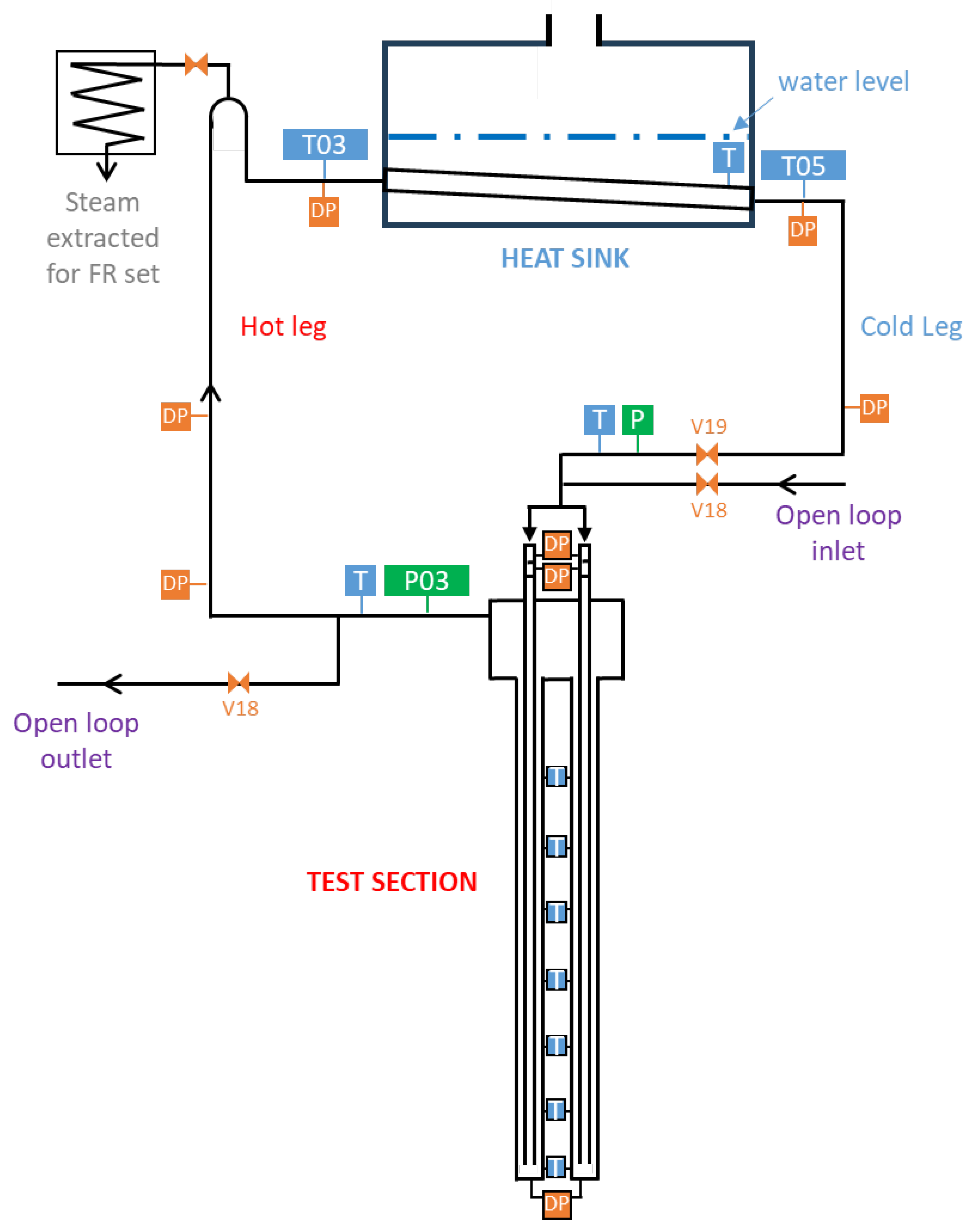
During the experimental campaigns, it was observed that the electrical heaters, which surround the external surface of the test section, gradually lose their sealing efficiency over time and thermal cycling, resulting in a reduced power supply compared to the value required for the specific test. Regarding the FR, at the beginning of each test, the loop is completely filled with water. To reach the correct conditions, a spill occurs along the hot-leg gooseneck, and the discharged tap water is manually weighed to determine the FR value. Although this procedure is simple to perform, it represents a significant source of uncertainty. Furthermore, considering the ratio between the maximum amount of water in the loop (about 20 kg) and the overall size of the facility, even small deviations in the operating parameters can play a relevant role in achieving the correct test conditions.

In order to extend the UA, based on engineering judgement, two other uncertainty parameters have been considered. One is the valve V19 concentrate loss coefficient; this component is fundamental for the correct operation of the system because its activation regulates the shift between the open-extended configuration and the closed-loop configuration. The assumption is the partial failure of the valve, which does not completely open, reducing the flow area. In order to simulate such phenomena, the key value selected for the analysis is the k-loss factor imposed on the valve flow area.

Finally, the air thermal conductivity within the gap between the central descending channel and the external annular channel of the test section has been considered, whose characteristics are not actually known.

The influence of these parameters on the determination of the facility operating conditions at a fixed FR and electrical power input was therefore examined and are evaluated in the subsequent uncertainty analysis.

6.1. Uncertainty Quantification Methodology

In order to better characterize model accuracy and gain key insights into the facility’s behaviour, a UA was performed, still considering the stationary closed-loop test CLOSE18.

In order to perform the UA, the GRS method [21] has been chosen. The first step of such methodology is the definition of the uncertainty parameter ranges and of the Probability Density Functions (PDFs); it envelops the state of knowledge of all the uncertainty parameters selected. Different types of uncertainty parameters can be chosen: input values (e.g., thermal conductivity of materials), model calibration values, boundary or initial conditions, and numerical values (e.g., min/max time step size). The nodalization uncertainty can be considered within the UA, adding different nodalization schemes to the analysis. Within the present work, such uncertainty has not been introduced in order to focus only on parameters related to the materials and test conditions.

Then, a sufficient number of simulation runs must be defined to ensure statistically meaningful results from the UA. In each simulation, all selected uncertainty parameters are varied simultaneously. The main advantage of this methodology is that it allows the application of statistical techniques in which the number of code runs is considered independent from the uncertainty parameters under investigation. As a result, a Phenomena Identification and Ranking Table (PIRT) is not required, since the ranking naturally arises from the analysis itself. The number of code runs depends on the selected probability content and confidence level of the statistical tolerance limits and is calculated according to the Wilks formula [22,23].

The uncertainty tool used to perform the present UA, for which the scheme of its logic is shown in Figure 17, was developed and applied thanks to a collaboration between the University of Palermo and the ENEA along the H2020 MUSA project [24], and it is a fully independent in-house tool written in Python 3. It was born for the MELCOR code application; however, within the present work, it has been adapted for R5 applications.

6.2. Results

Such work aims to perform a UA in order to collect key insights on the facility behaviour, on the statistical correlation between the input uncertainty parameters selected, and the Figures of Merits (FOMs).

Following several past works [5,25], the first step of the UA is the selection of the FOMs; in particular, within this work, the selected ones are as follows:

• HX exchanged power—FOM_1;
• The pressure in the VC (P03)—FOM_2;
• The loop mass flow rate—FOM_3.

The three FOMs selected are the key indicators to evaluate the capability of the plant to perform the safety action required. In order to propagate the uncertainty among the selected FOMs, a set of uncertainty input parameters must be defined. In

Table 4. Uncertainty parameters’ range definition.

Parameter	Unit	PDF	Reference Value	Lower/Upper Bound		Reference
Filling Ratio	kg	Normal	13.654	Max	+10.0%	Engineering Judgement
				Min	−10.0%
Electrical Power	kW	Normal	27.9	Max	0.0%	Engineering Judgement
				Min	−15.0%
V19 loss coefficient	-	Normal	0.03	Max	+100.0%	Engineering Judgement
				Min	−100.0%
Gap Air conductivity	${\displaystyle \frac{\mathrm{W}}{\mathrm{m}·\mathrm{K}}}$	Normal	0.05	Max	+5.0%	Engineering Judgement
				Min	−5.0%

, there is an explanation of the defined PDF applied for each input parameter, the type of PDF used, and the lower/upper bound of the selected range.

Considering the Wilks formula [22,23], 124 runs were needed to reach probability $\mathsf{\gamma }$ and a confidence level $\mathsf{\beta }$ of 95% for each FoM; therefore, in order to be more conservative and considering possible run failures, 150 runs were considered in the analysis.

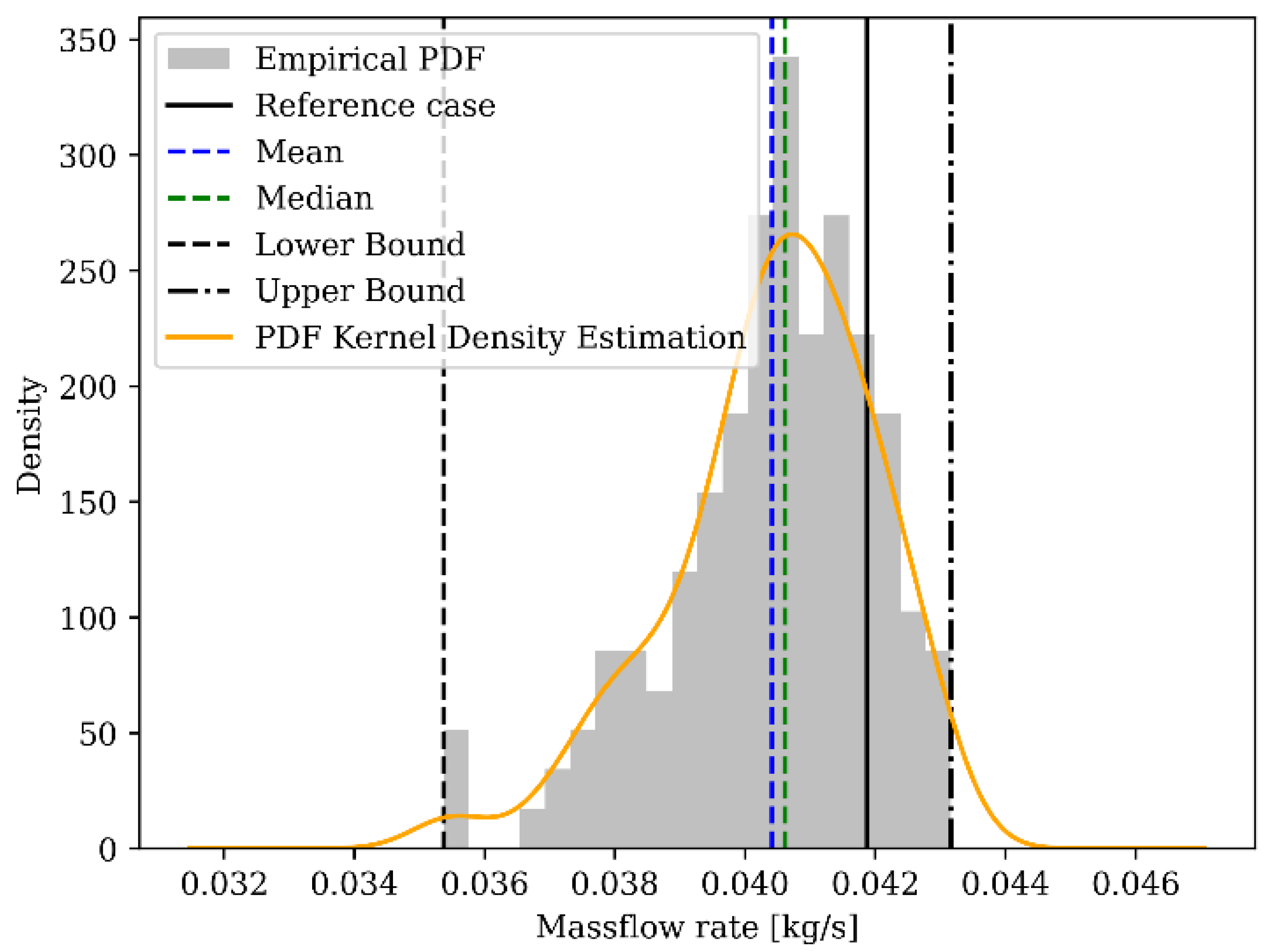
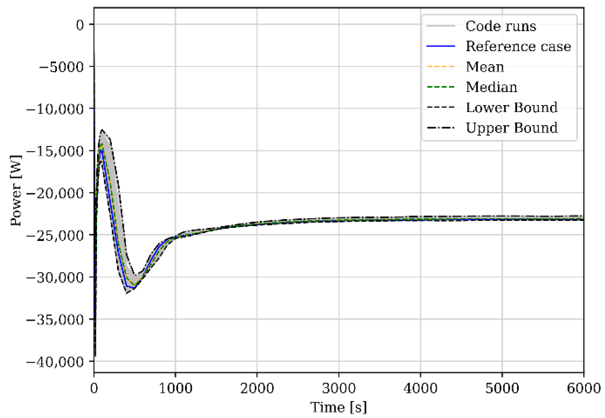
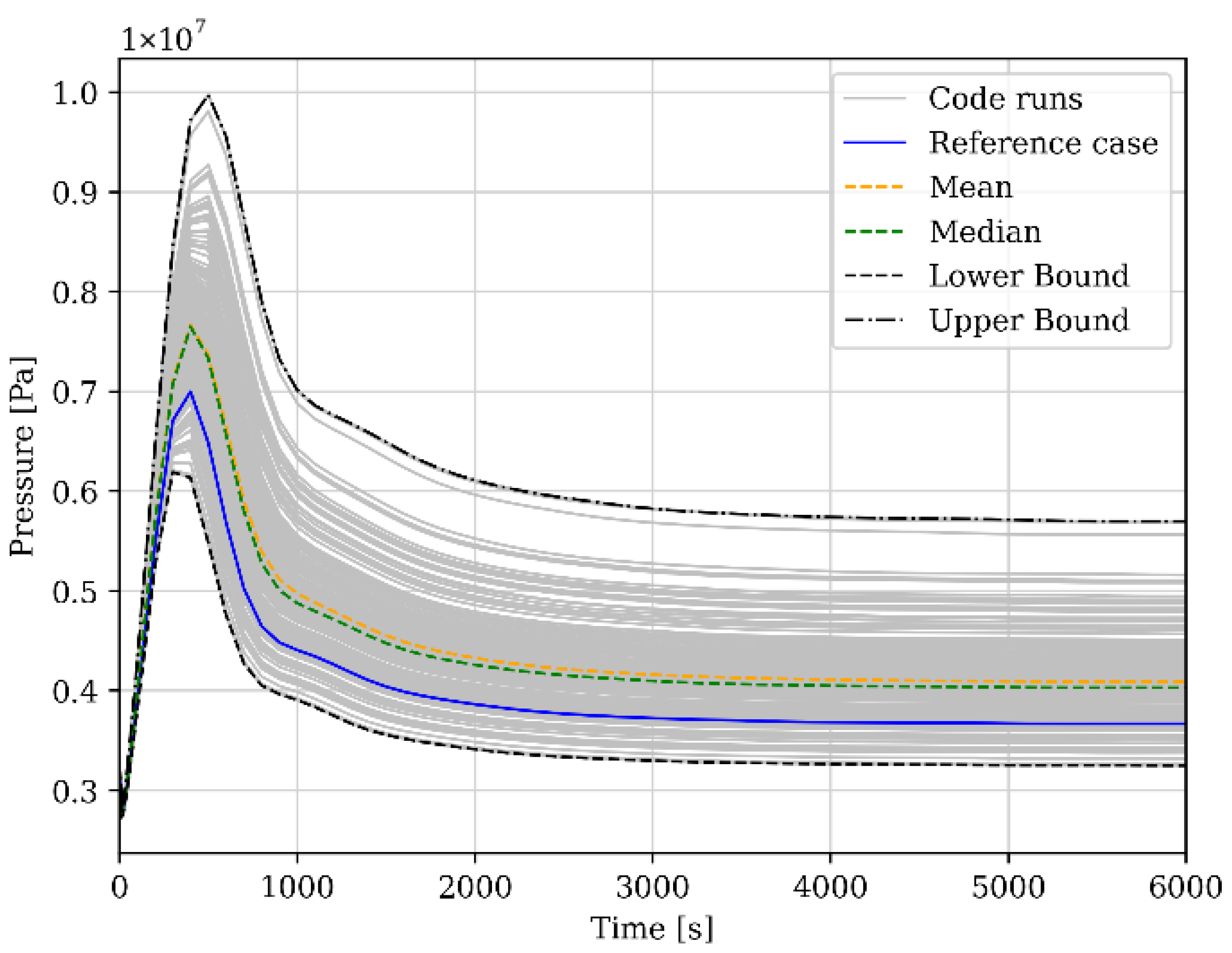
Figure 18, Figure 19 and Figure 20 represent the calculated PDF of the FOMs compared to the reference code calculation (the CLOSE18 test with all the reference values for the selected uncertainty parameters) and the calculated statistical parameters, such as the mean, median, and lower and upper bound.

In

Table 5. Characteristic values of the FOMs’ calculated PDFs.

	FOM_1	FOM_2	FOM_3
	HX Power [W]	VC Pressure [Pa]	Mass Flow Rate [kg/s]
Mean	−2.3070 × 104	4.0893 × 106	0.0404
Median	−2.3071 × 104	4.0289 × 106	0.0406
Lower bound	−2.3255 × 104	3.2492 × 106	0.0354
Upper bound	−2.2752 × 104	5.6973 × 106	0.0432
Coefficient of variation	−0.4%	11.4%	3.9%
Kurtosis	0.17	1.31	0.70
Skewness	0.52	0.93	−0.80

all the numerical values related to the mean, median, and lower and upper bound are represented; moreover, the kurtosis parameter, indicating the “extremeness” of the distribution tails compared to a normal distribution, and the skewness parameter, indicating the symmetry of the data’s distribution compared to the mean, are represented [26].

The joint analysis of mean, median, skewness, and kurtosis reveals the underlying nature of the data: where they are concentrated, how they are distributed, and how predictable they are, giving more information about the uncertainty.

All the considerations are summarized in

Table 6. Characteristic statistical parameters.

	FOM_1	FOM_2	FOM_3
	HX Power [W]	VC Pressure [Pa]	Mass Flow Rate [kg/s]
Mean and Median	Practically equal	Higher mean	Practically equal
Coefficient of variation	No variation	Relevant variation	Minimum variation
Skewness	Symmetric	Longer right tail	Slightly longer left tail
Kurtosis	Mesokurtic	Leptokurtic	Leptokurtic

.

Observing Table 6 and focusing on the FOM_1 column, it is possible to detect that the accuracy of the central value is high and the distribution of the population’s assumed values is practically equal to the mean value; moreover, the value of the skewness and kurtosis parameters guarantees a symmetrical normal distribution. For these reasons, the expected range of uncertainties is small, as shown in Figure 21. Similarly, even with some discrepancies and not properly symmetric behaviour, the same expected range behaviour is predicted for the loop mass flow rate (FOM_3) as shown in Figure 22. On the contrary, the VC pressure (FOM_2) highlights a non-normal distribution with a consistent difference in the central value; moreover, by observing the skewness and the kurtosis coefficient, it is possible to understand that the PDF has a lower value than the mean value and is closer to the reference value; however, it has an extreme outlier higher than the reference calculation’s value. Therefore, for these reasons, the expected variation range of such an FOM is larger than the other FOMs’ ranges, as shown in Figure 23.

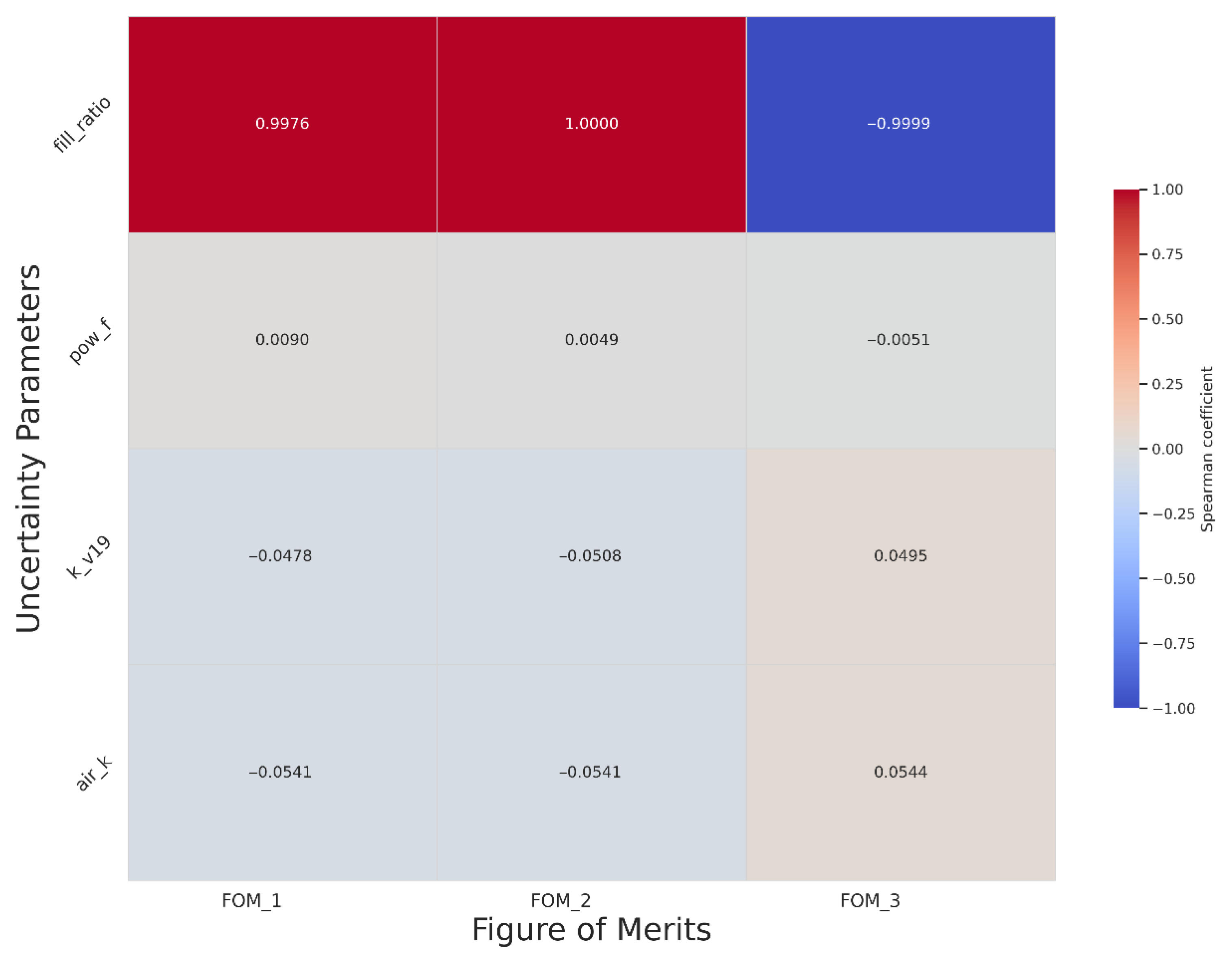
The Spearman’s correlations for each FOM related to each uncertain input parameter have been calculated. In Figure 24, Spearman’s heat map is represented. The colour represents the intensity and the direction of correlation (red indicates positive correlation, while blue a negative correlation).

From the statistical correlation analysis, it emerges that all three FOMs present a high statistical correlation with the filling ratio. In particular, there is a positive correlation with respect to the HX power and the VC pressure and a negative correlation with respect to the mass flow rate. On the contrary, the other parameters, compared to the selected FOMs, present a non-significant statistical correlation.

The meaning of such considerations is that the system is very sensitive to small variations in the filling ratio at the beginning of the stationary test because it can alter the amount of water in the loop, changing the density gradient, the void fraction distribution, and, therefore, the VC pressure behaviour, altering the thermal-hydraulic condition of the test.

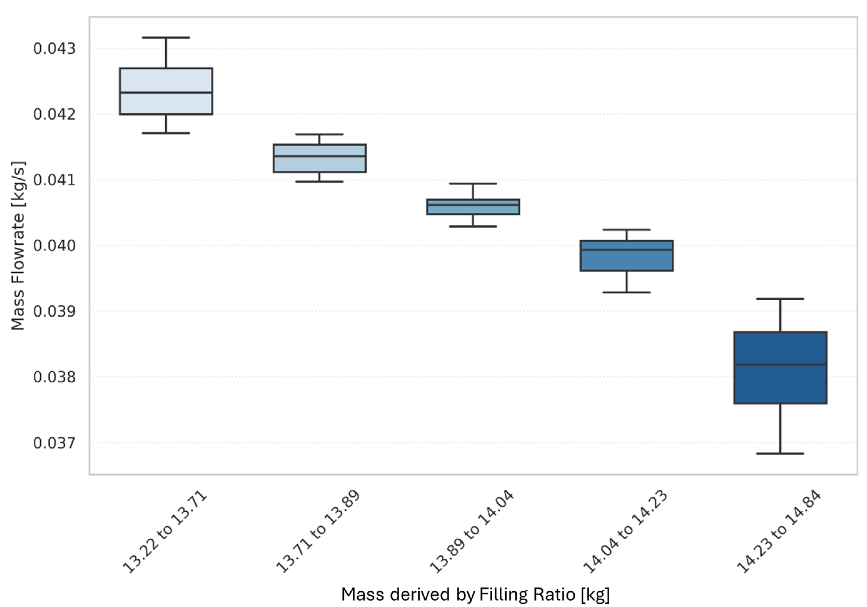
Based on the Spearman results, additional considerations can be performed; in particular, such correlation coefficients determine the degree of a monotonic relationship, if it exists, between two variables but do not indicate for which specific value in the sampled parameter population the uncertainty of the FOMs is higher. Therefore, considering the filling ratio as the only parameter to better analyze due to the high statistical correlation, five groups of such parameter’s values were defined and used in Figure 25, Figure 26 and Figure 27 to create box plots. In particular, the box plot visually summarizes the distribution of a dataset through five key elements: the median (central line), the InterQuartile Range (IQR), which is the box spanning the 1st quartile and 3rd quartile, the whiskers, representing the minimum and maximum value (extending to 1.5 × IQR), and outliers (individual points beyond the whiskers).

In Figure 25, the box plot representing the FOM_1 HX power dataset in relation to the filling ratio is presented. Observing the five groups, it can be observed that for the filling ratio value groups 13.22–13.71 and 13.89–14.04, there is low variability compared to the central data, especially for the value group 13.89–14.04, where the population within the first and third quartiles is close to the median.

On the other hand, for the value groups 13.71–13.89 and 14.23–14.84, the IQR is very wide, showing a more dispersed distribution further from the median. Therefore, it can be said that, concerning HX power, for high filling ratio values within the sampling range, the uncertainty is high compared to the other groups. On the other hand, even though this is the group with the greatest uncertainty among the five considered, looking at the numerical values of the power, it is possible to observe that, on a practical level, there are minimal variations in power, as also found by observing the range of variation in Figure 21.

Regarding the dataset relating to FOM_2 VC pressure, shown in Figure 26, it can be observed that the three central groups have a small IQR with values close to the median and also maximum and minimum values very close to the IQR, meaning that for these filling ratio values, the uncertainty relating to the population is very limited. However, looking at groups 13.22–13.71, representing the range with the minimum values, and 14.23–14.84, representing the range with the maximum sampled filling ratio values, it is possible to observe a significant variation in the IQR with, especially for the range 14.23–14.84, long whiskers of varying lengths, indicating high data dispersion and asymmetry in the distribution of the dataset. The range of variation in the two critical intervals is approximately 5–6 bar, indicating significant uncertainty regarding the determination of the saturation conditions of the system and, therefore, of the thermohydraulic conditions of the water within the loop.

Lastly, considering the FOM_3 mass flow rate, shown in Figure 27, and observing the entire spectrum of its variation, it can be observed that the range of uncertainty is minimal, as also shown in Figure 20. In any case, it is possible to focus on the range with the highest values (14.23–14.84), noting the highest dispersion and also an asymmetry in the distribution of mass flow values tending towards the minimum value of the distribution. In addition, it can be observed that as the filling ratio value increases, the trend of the FOM values is negative. This is explained by the fact that the more water is present in the loop, the more the density gradient needed to provide motion to the fluid decreases, decreasing the mass flow rate.

7. Conclusions

The safety and reliability of NPPs are fundamental for the development of nuclear energy, requiring continuous improvements in safety assessments and accident simulations. Passive safety systems have emerged as a promising solution to enhance safety standards; however, their reliability remains a critical area of investigation, particularly during activation and under specific T/H conditions.

To accurately predict the behaviour of such systems during accidental scenarios, validated system codes such as R5 must be updated and refined to properly account for passive system dynamics, including specific phenomena such as heat transfer in the presence of NCGs, condensation on containment structures, etc.

In this work, the RELAP5 code has been modified with the implementation of Thome’s correlation for the simulation of condensation phenomena in horizontal pipes, replacing the Chato–Shah correlation model used in the standard code. The implementation required an in-depth study of the internal structure of RELAP5, in particular the logic that rules the individual simulation process. Subsequently, the new modified code version was used to perform a new calibration of the input deck for the HERO-2 facility, to carry out a sensitivity study of the model considering the SAF parameter on the HX section, and finally to perform the simulation of 24 steady-state tests in natural circulation.

The obtained results have shown that, unlike previous studies, it is not necessary to recalibrate the heat exchange coefficient when switching from extended open-circuit tests to closed-circuit tests. For this reason, the comparison between the numerical results and the experimental data shows a slight improvement compared to the results obtained previously, confirming the overestimation of the natural circulation mass flow rates, derived from the general underestimation of the temperatures in the cold leg and therefore an overestimation of the driving force.

To assess the potential uncertainty related to the experimental data used to validate the new R5 model, a UA was performed by selecting specific uncertainty parameters based on engineering judgement. The GRS method [21] was applied followed by a statistical evaluation of the results. The analysis showed that the parameter with the greatest influence on the selected FOMs is the filling ratio, which represents an initial condition for all 24 steady-state closed-loop tests. Even small variations in the FR, on the order of a few grams of water, given the limited size of the facility, can significantly affect the specific test parameters and alter the intended conditions.

Consequently, it is difficult to quantify the extent to which either the new or the standard version of RELAP5 overestimates the driving forces in the loop. In particular, while the updated code version demonstrates a modest improvement in calibration, it does not show any substantial enhancement in the overall simulation accuracy. Since the measurement of the filling ratio is affected by considerable uncertainty, reducing this variability remains essential to improving the code’s predictive performance.

However, it should be emphasized that the application of this version of the code to the experimental tests conducted at the HERO-2 facility cannot be considered sufficient to evaluate its actual simulation capabilities. Nevertheless, it can be concluded that the objective of this work has been achieved, leading to a version of the RELAP5 code that includes a dedicated correlation for condensation in horizontal pipes, which provides a more realistic representation of the condensation phenomena in a broader range of operating conditions. Further evaluations can be performed in future activities with the application of the modified code to the simulation of experimental data from other facilities.