SNM Radiation Signature Classification Using Different Semi-Supervised Machine Learning Models

Abstract

The timely detection of special nuclear material (SNM) transfers between nuclear facilities is an important monitoring objective in nuclear nonproliferation. Persistent monitoring enabled by successful detection and characterization of radiological material movements could greatly enhance the nuclear nonproliferation mission in a range of applications. Supervised machine learning can be used to signal detections when material is present if a model is trained on sufficient volumes of labeled measurements. However, the nuclear monitoring data needed to train robust machine learning models can be costly to label since radiation spectra may require strict scrutiny for characterization. Therefore, this work investigates the application of semi-supervised learning to utilize both labeled and unlabeled data. As a demonstration experiment, radiation measurements from sodium iodide (NaI) detectors are provided by the Multi-Informatics for Nuclear Operating Scenarios (MINOS) venture at Oak Ridge National Laboratory (ORNL) as sample data. Anomalous measurements are identified using a method of statistical hypothesis testing. After background estimation, an energy-dependent spectroscopic analysis is used to characterize an anomaly based on its radiation signatures. In the absence of ground-truth information, a labeling heuristic provides data necessary for training and testing machine learning models. Supervised logistic regression serves as a baseline to compare three semi-supervised machine learning models: co-training, label propagation, and a convolutional neural network (CNN). In each case, the semi-supervised models outperform logistic regression, suggesting that unlabeled data can be valuable when training and demonstrating value in semi-supervised nonproliferation implementations.

1. Introduction

1.1. Motivation

Through a set of tools and technologies, organizations such as the International Atomic Energy Agency (IAEA) monitor nuclear activity and ensure that nation states or individuals are abiding by laws, regulations, and international agreements. The Atomic Energy Act of 1954 (AEA) defines SNM as "plutonium, uranium enriched in the isotope 233 or in the isotope 235, and any other material which the Commission…determines to be special nuclear material [1]". The illicit use of SNM and other radioactive materials therefore necessitates timely detection and characterization—important steps toward ensuring nuclear nonproliferation.

This can be a difficult objective to achieve without prior knowledge of the event itself. Confounding variables and complex physical behavior can occlude radiation signatures associated with SNM transfers or confuse models based on advanced computing techniques such as machine learning (ML). Many established ML implementations require large volumes of data and/or significant computing costs for pattern recognition. Abundant data and computing resources may not apply in nuclear nonproliferation scenarios where an increased burden on verification with limited resources [2] necessitates resource efficiency. The primary motivation of this work is to focus on tools that can be employed to distinguish SNM transfers from other environmental effects. This involves answering the following: (1) is a nuclear material transfer occurring, (2a) what kind of material is it, and (2b) how much material is present? Achieving both objectives without prior knowledge unique to the transfer event is essential, provided that the implementation alleviates the high computing and domain costs typical for traditional ML methods.

Without precise contextual information, signatures from a material transfer may be difficult to resolve with rudimentary detection algorithms or can be prone to misidentification. Thus, the cost of labeling training data needed for appropriately generalizable models can be as prohibitive as manually evaluating measurement samples with a subject-matter expert (SME). Methods employing semi-supervised machine learning (SSML) attempt to address this by incorporating unlabeled data to achieve a performant model with the limited labeled data expected in constrained resource scenarios. As shown herein, accuracies competitive with supervised methods are observed when the volume of unlabeled data is much larger than the volume of labeled data, making semi-supervised machine learning worthwhile when labeled data are costly to produce, rare, or limited in volume. This means that monitoring institutions can still utilize information gathered even if it has not been extensively labeled.

1.2. Semi-Supervised Applications to Nuclear Engineering

Most applications of semi-supervised machine learning in nuclear engineering to date have been for fault diagnosis and transient identification. Ma and Jiang [3] utilize a graph-based SSML method. This is implemented in a self-training workflow, incorporating new data in future training iterations. Empirical success was shown in classifying experimental and simulated nuclear power plant (NPP) fault scenarios. Another example of SSML used for nuclear safety is Pinciroli et al. [4], where a more ad hoc system of feature extraction based on importance for characterization is used. Sun et al. [5] use a system of weak supervision to implement a convolutional neural network (CNN) that applies pseudo-labels eventually included in future training. This results in a system for object detection that then is applied to nuclear waste.

Moshkbar-Bakhshayesh et al. [6,7] use a two-step approach for identifying transients and then apply SSML to unknown transient classifications. First, a supervised machine learning model attempts to identify known transients. Unknown transients are then passed to a transductive support vector machine (TSVM) to predict unlabeled samples.

In general, these papers present implementations of SSML to nuclear engineering that demonstrate viability but lack context to nuclear nonproliferation. Implementations of SSML appear to be an emerging technology for nuclear nonproliferation applications. Most applications of machine learning in this space are supervised, which do not utilize the plethora of unlabeled data that may be available when labeling is costly. Therefore, SSML should be tested as a viable alternative to supervised machine learning techniques.

1.3. Goals

This work evaluates how semi-supervised machine learning can utilize information gained from both unlabeled and labeled data in pattern recognition algorithms for application in nuclear nonproliferation. In this application space, the goal is to optimally leverage large volumes of radiation data with limited ground-truth data. The efficacy of SSML models will be demonstrated on real-world data collected at Oak Ridge National Laboratory (ORNL) containing transfers of shielded radiological material. Previous implementations that utilize Multi-Informatics for Nuclear Operating Scenarios (MINOS) data have relied on anomaly detection using a sequential probability ratio test (SPRT) with post hoc data analysis [8] or physics-informed machine learning combined with data fusion [9].

Here, an alternative method with careful consideration of human and computing costs is offered. The model presented can detect anomalous radiation measurements and, when trained, uses a machine learning method to distinguish transfers from other anomalous events. A hypothesis testing algorithm is implemented in order to identify anomalies. This test is also used to determine the domain-specific thresholds for anomaly detection. The results are fed into a labeling heuristic that applies a pseudo-label that is then used for training and testing various machine learning models. Overall, three SSML implementations are benchmarked against one supervised method. The results indicate an advantage in using an SSML method that utilizes unlabeled data when labeled data are limited.

In summary, the main contribution of this work is an empirical demonstration of SSML as a tool for nuclear nonproliferation. The workflow introduced here utilizes all data collected, regardless of labeling status, without sacrificing performance but rather improving it over comparable supervised methods.

2. Background

2.1. Machine Learning Overview

Writ large, machine learning, or artificial intelligence, are sets of statistical methods typically used to describe nonlinear, physical systems, sometimes using experimental observations to guide construction. This introduction reflects much of the reasoning, and further information can be found in the textbook by Shalev-Shwartz and Ben-David [10]. Other overviews can be found in textbooks by Russell and Norvig [11] (which include discussions on implementation) or by Devroye et al. [12] (with a slightly more statistical perspective). This work’s scope is limited to machine learning used for classification. Observed instances, x, are sampled from a distribution, $P\left(\mathcal{X}\right)$, determined by domain-specific physical processes. A single instance is typically represented as a feature vector of discrete elements that could be sampled from continuous nonlinear systems. Examples include (but are not limited to) images, mathematical variables, spectra, health data, etc.

For a given $x\sim P\left(\mathcal{X}\right)\in {\mathbb{R}}^d$, the goal of machine learning is to find a function that relates this to a label, $y\sim \mathcal{Y}$. The set of classes, $\mathcal{Y}$, defines the possible labels for the modeled system. The set of datapoint instances, $\mathcal{X}$, can take many forms depending on the input modality and the model being designed. Said another way, ML methods find a relationship between x and y such that the model, f, can approximate the relationship: $f\left(x\right)\approx y\forall (x,y)\in (\mathcal{X},\mathcal{Y})$. For example, the model could be trying to classify good versus bad fruit, in which case, the labels may be good banana, bad banana, good apple, or bad apple, and the instances could be observations of individual pieces of fruit (e.g., color, shape, size).

To do this, some observations must be used. Labeled instances, L, used in "supervised" machine learning, have an associated label, and the total number of paired instances is $n=\left|L\right|$. If observations are present without labels, it is possible to perform "unsupervised" machine learning on this unlabeled dataset, U, numbering $m=\left|U\right|$ instances. The observed dataset distribution consists of both forms:

$$\mathbb{D}=\{(x_1,y_1),(x_2,y_2),\dots ,(x_{\left|L\right|},y_{\left|L\right|}),x_{\left|L\right|+1},\dots ,x_{\left|L\right|+\left|U\right|}\}.$$

(1)

For supervised learning, this culminates in empirical risk minimization (ERM) using a loss function. The loss function is some form of penalization against misclassification of known observations: $\frac{1}{n}{\sum }_{i=1}^n\mathcal{L}(f\left(x_i\right),y_i)$. There may be many, even infinite, models that describe the observed system. The goal is therefore to find the optimal model that minimizes this loss function:

$$\widehat{f}=\underset{f}{argmin}\frac{1}{n}\sum _{i=1}^n\mathcal{L}(f\left({\mathit{x}}_i\right),y_i).$$

(2)

There are many ways to choose the model, the loss function, the method of finding $\widehat{f}$, or even the instances $({\mathit{x}}_i,y_i)$ used. A simple model would be a linear regression system where each feature vector, ${\mathit{x}}_i=[x_1,x_2,\dots ,x_j]$, is connected to its label, $y_i$, by a system of weights, $\mathit{w}$. Then, the model becomes $f\left({\mathit{x}}_i\right)={\widehat{y}}_i={\mathit{w}}^{⊺}{\mathit{x}}_i+b$ where b is a bias term. The loss could then be a mean square error (MSE), and ERM finds the optimal set of weights that describes all $({\mathit{x}}_i,y_i)$ with minimal loss:

$$\widehat{\mathit{w}}=\underset{\mathit{w}}{argmin}\sum _{i=1}^n{({\mathit{w}}^{⊺}{\mathit{x}}_i-y)}^2.$$

(3)

2.2. Semi-Supervised Machine Learning

Semi-supervised machine learning encompasses ML models that use both labeled and unlabeled data. This class sits between traditional supervised and unsupervised machine learning. The development of these methods was motivated by high-cost regimes for labeling. In some fields, labeling must be carried out manually and requires domain expertise. Both methods increase the cost of this time-consuming pre-processing step. When the cost is prohibitive, but data are plentiful, SSML can be useful. For a larger overview of SSML, refer to the textbook compiled by Chappelle et al. [13]. Semi-supervised learning relies on certain assumptions to learn a decision boundary. That is, the learned mathematical description that separates classes is in the feature space. This is necessary for connecting information about classification from labeled data to knowledge about the underlying data distribution from unlabeled data.

The cluster assumption states that if two samples, $x_1$ and $x_2$, are close together, their labels should agree: $y_1=y_2$. The notion of closeness is up to interpretation and depends on the unique data modality. If true, selected features describe the state space responsible for classification with some notion of smoothness, i.e., $f(x_0\pm ϵ)$ should exhibit the same response for some small noise, $ϵ$. A model cannot learn a decision boundary from a feature vector if the feature space has no correlation with class labels. This is connected to the smoothness assumption, which contends that classes of data should be clustered in a region of high density that is describable by that state space.

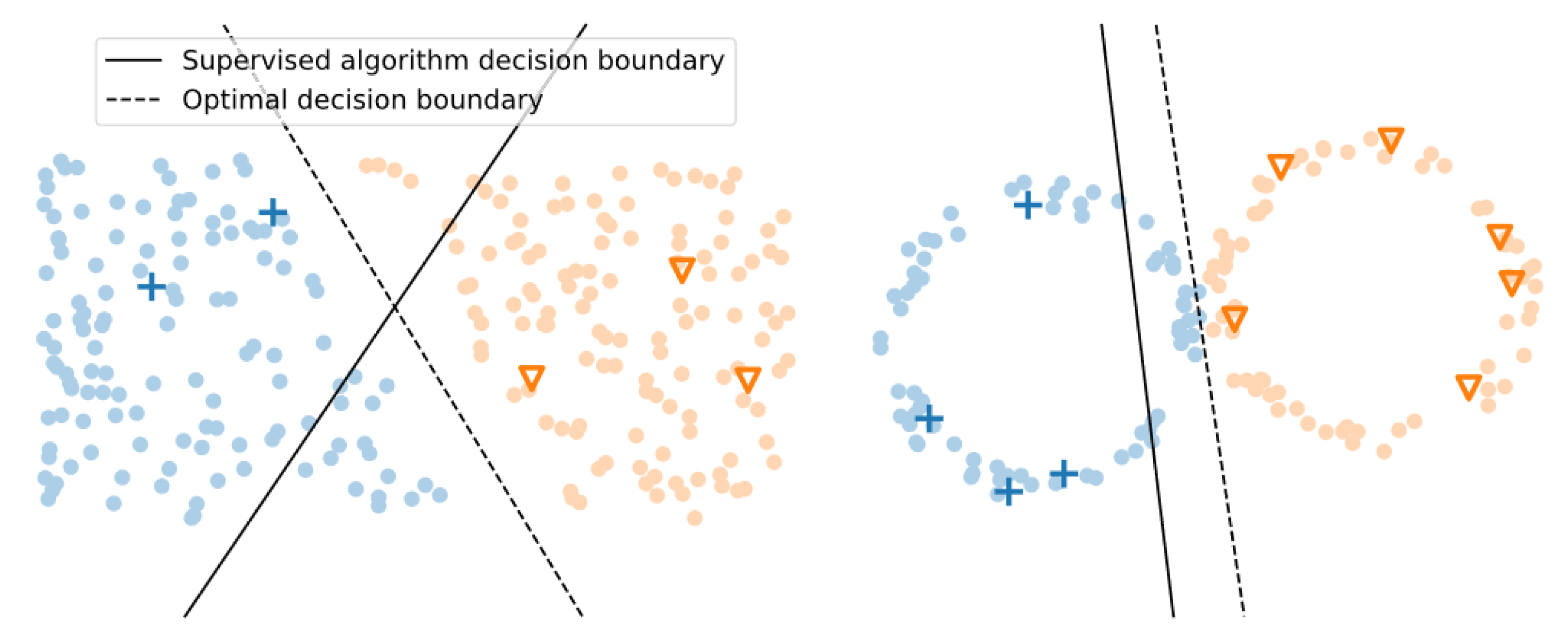
The manifold assumption maintains that higher-dimensional data lie on a lower-dimensional manifold (a topological space). Therefore, the decision boundary that separates classes in this space may also be lower dimensional and thus does not require the entire feature space to discern separation. For example, a three-dimensional dataset may have a two-dimensional representation that makes its classes separable. Both assumptions are illustrated in Figure 1. Each assumption supports scenarios in which unlabeled data can improve a learned decision boundary with added information.

T. Lu [14] argues that near certainty about "some non-trivial relationship between labels and the unlabeled distribution" is required for success with SSML. Otherwise, convergence will not be guaranteed. Singh, Nowak, and Zhu [15] take this further by quantifying the data distribution contexts in which SSML will converge faster or perform better than supervised methods (particularly when $m\gg n$). This is carried out within the perspective of the cluster assumption, but the definitive conclusion agrees with the above: SSML will be more effective if a relationship exists and if classes are sufficiently distinguishable. Arguably, this holds for nuclear radiation data. Spectra that come from the same radiation source should exhibit the same radiation signature/photopeak. Any variation is the result of environmental effects and detector efficiencies such as distance to source and the overall underlying background distribution. Spectra should contain the same labeling information regardless of whether they are labeled or unlabeled, excluding edge cases where the signature is barely discernible within a spectrum (such as border samples from Singh et al. [15]).

Figure 1. The two underlying SSML assumptions include the cluster assumption (left) and the manifold assumption (right). In each plot, pluses and triangles are labeled instances, and dots are unlabeled instances. Colors (blue and orange) represent different classes. Note how the inclusion of unlabeled data in a ML model would improve its learned decision boundary. (Image source: [16]).

Figure 1. The two underlying SSML assumptions include the cluster assumption (left) and the manifold assumption (right). In each plot, pluses and triangles are labeled instances, and dots are unlabeled instances. Colors (blue and orange) represent different classes. Note how the inclusion of unlabeled data in a ML model would improve its learned decision boundary. (Image source: [16]).

3. Methods

3.1. MINOS Data

The MINOS venture at ORNL collects multi-modal data streams relevant to nuclear nonproliferation. This is accomplished using a network of nodes distributed at ORNL’s campus surrounding two points of interest: the Radiochemical Engineering Development Center (REDC) and the High-Flux Isotope Reactor (HFIR). The reactor facility, HFIR, is used for scientific experiments (e.g., neutron scattering) and isotope production. Materials generated at HFIR are loaded into shielded casks and are transferred by flat-bed truck to REDC. Once at REDC, the materials are unloaded, stored, and/or processed in, for example, hot cells.

Some of the material produced and processed at ORNL and detected by MINOS include [9]:

• Unirradiated ²³⁷Np targets used for ²³⁸Pu production;
• Irradiated ²³⁷Np containing ²³⁸Pu;
• Unirradiated Cm targets used for ²⁵²Cf production;
• Irradiated Cm containing ²⁵²Cf;
• ²²⁵Ac;
• Activated metals;
• Spent fuel.

The ultimate goal is to develop capabilities that distinguish and differentiate between shielded radiological material that might be present at the testbed. Material transportation can occur along several routes between facilities. Nodes in MINOS are distributed across the possible routes alongside the road. These nodes collect different forms of data including atmospheric conditions (e.g., temperature and pressure), video, audio, seismo-acoustic, and radiation.

Radiation data are collected using a network of sodium iodide (NaI) detectors—each designated as a node—that are distributed along the roads between HFIR and REDC. This detector is capable of measuring gamma radiation emitted from nearby sources. Nodes are designed to take one measurement every second. This measurement is energy-dependent, binned in 1000 channels of 3 keV per bin. Energy calibration, which accounts for gain drift in detector electronics, is completed before being shared for data analysis. Materials transferred around the MINOS testbed will serve as observables for developing and testing analysis methods.

3.2. Nuclear Material Transfers

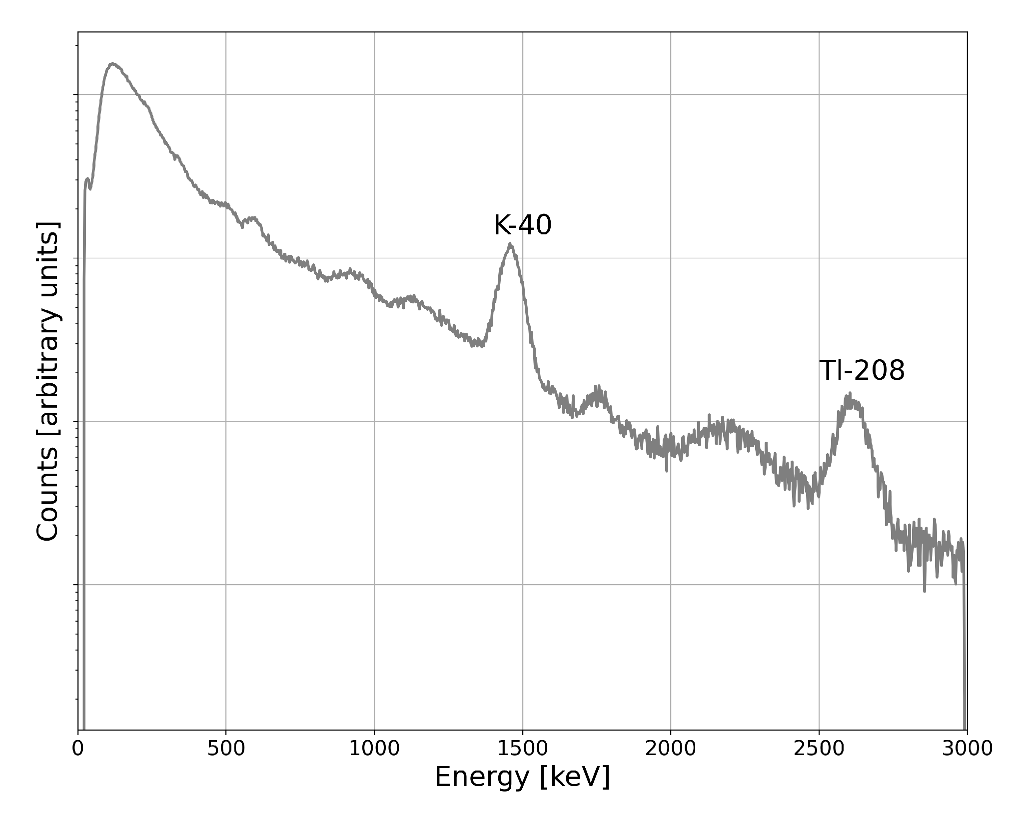
One method of detecting shielded radiological material transfers would be with radiation monitoring. An example gamma radiation spectrum can be seen in Figure 2. Some photopeaks visible in the spectrum are the result of persistent background radiation that naturally occurs around Earth. This includes signatures related to the potassium–uranium–thorium (KUT) continuum (⁴⁰K and ²⁰⁸Tl, for example). Other signatures present in the spectrum must be measured and identified. 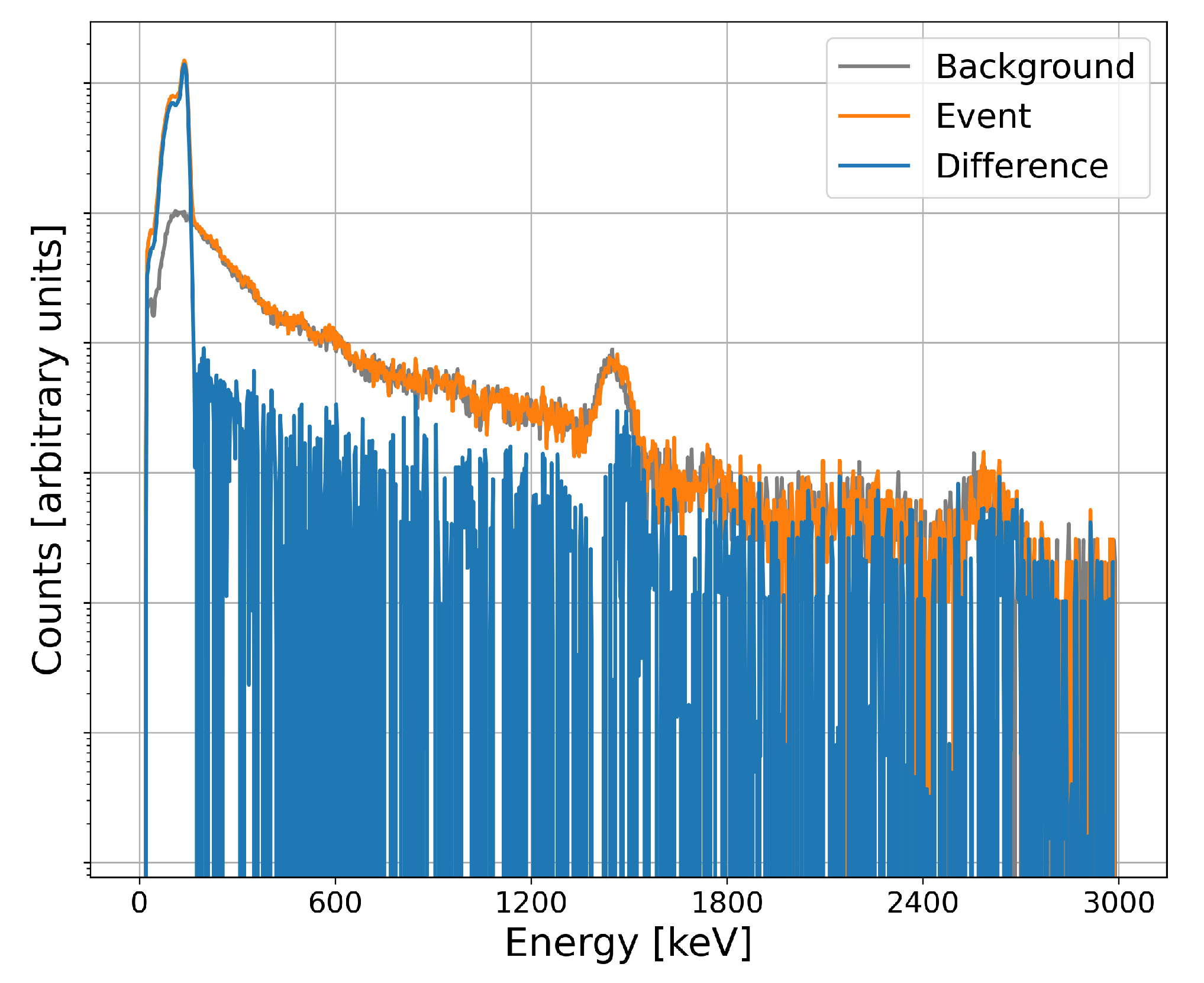Figure 3 is a spectrum taken during a material transfer. To accentuate the portion of the spectrum that is associated with the material transferred, a portion of the background has been estimated and subtracted (blue line). Note the substantial increase in count-rate at low energies. This continuum is the result of radiation from the transferred material being downscattered by container shielding. In this case, for example, a detection model must be trained to identify this response and associate it with the appropriate radiation event type.

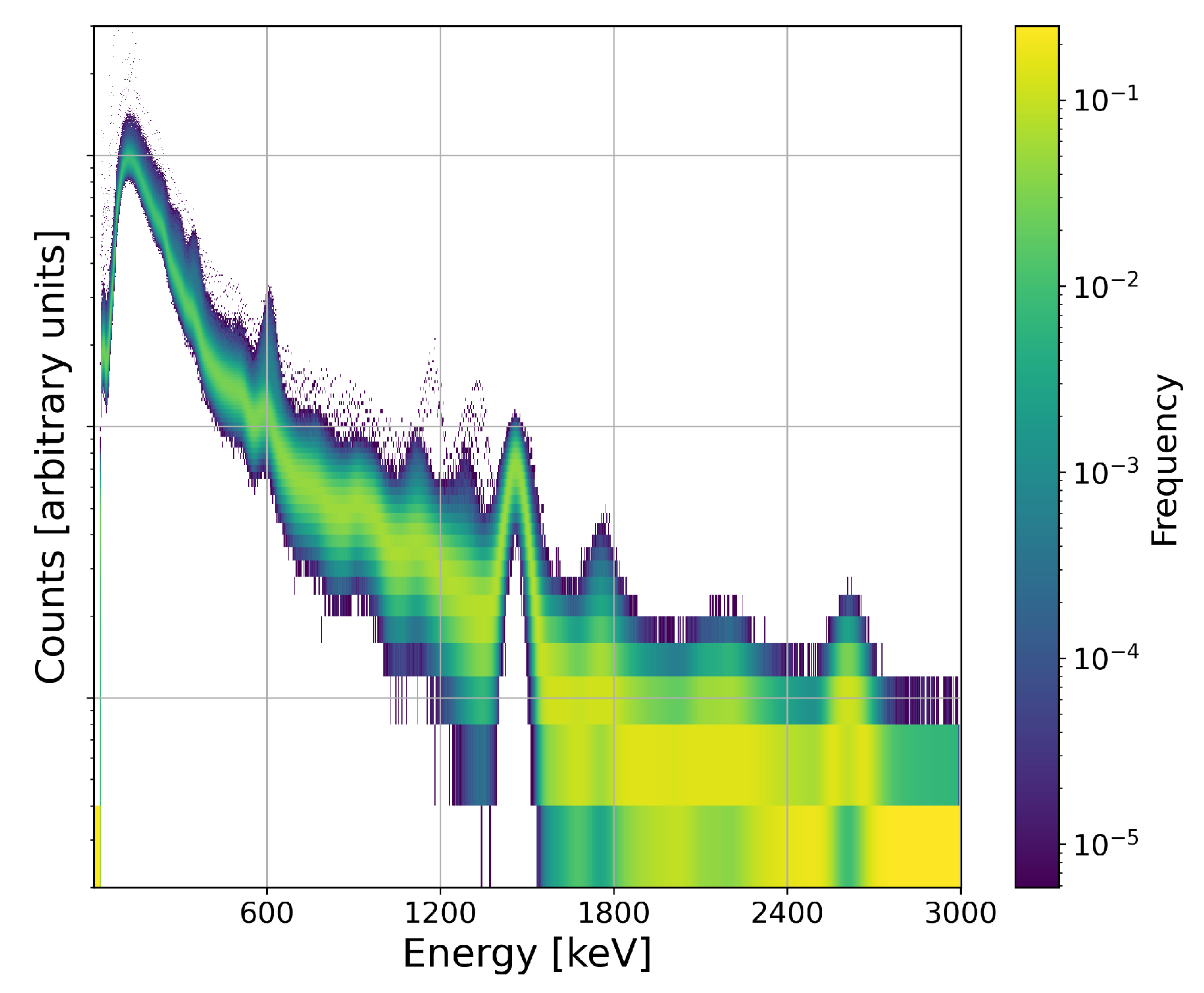
Radiation measurements are temporal, meaning they can be continuously measured and will vary statistically with time. One month of 1-minute measurements are plotted in Figure 4. A normalized frequency histogram is plotted in each energy bin of the plot. That means that each vertical slice is a frequency of how often the measurement for that energy bin registered that magnitude of count-rate over the course of the month. The goal of this work is to identify anomalous measurements outside of the typical distribution represented in yellow and green. The low energy signatures associated with transfers are visible as small purple dots, as well as other off-normal measurements elsewhere in the energy spectrum.

3.3. Radiation Events

A transfer event occurs when a vehicle or source moves past a detector and thereby exhibits a response in that node. Material recently generated in HFIR will typically have high activity, which is why shielding is necessary for the safety of individuals handling the material. This shielding means that the signature’s characteristic photopeak will not be observed by the detector. Instead, emitted gammas are scattered by the shielding material before reaching the detector. The NaI response will appear as a low-energy, downscattered continuum without the expected photopeak. If a background spectrum can be measured or approximated, this continuum should appear above the characteristic background. This is time dependent, and count rates will rapidly rise as the transportation vehicle approaches and fall as it drives past the detecting node.

Other radiation events can appear to be anomalous if they exhibit similar rapidity in count-rate change and must be accounted for in detection algorithms. For example, HFIR produces a large flux of neutrons when it is active. These neutrons can be captured by argon naturally in the air at a non-negligible rate. This produces ⁴¹Ar, which is radioactive, undergoing ${\beta }^{-}$ decay to stable ⁴¹K while emitting gamma radiation with a photopeak energy of 1294 keV. Another example occurs when it rains, which can "washout" radioactive ²²²Rn with a half-life of approximately 3.8 days and is a result of the decay of ²³⁸U. This weather pattern will exhibit elevated gamma radiation sourced from the radioactive daughters in this decay chain.

These unique environmental conditions will each contribute to the background radiation distribution with different intensities at different times. Exact characterization of the background spectrum is impossible without full knowledge of these conditions. Even a fully constructed background distribution for one measurement may not be transferable to a second measurement with different diurnal or seasonal variations. Here, an estimation of background is used if it is reasonable for a given time and state of a measurement.

3.4. Hypothesis Testing

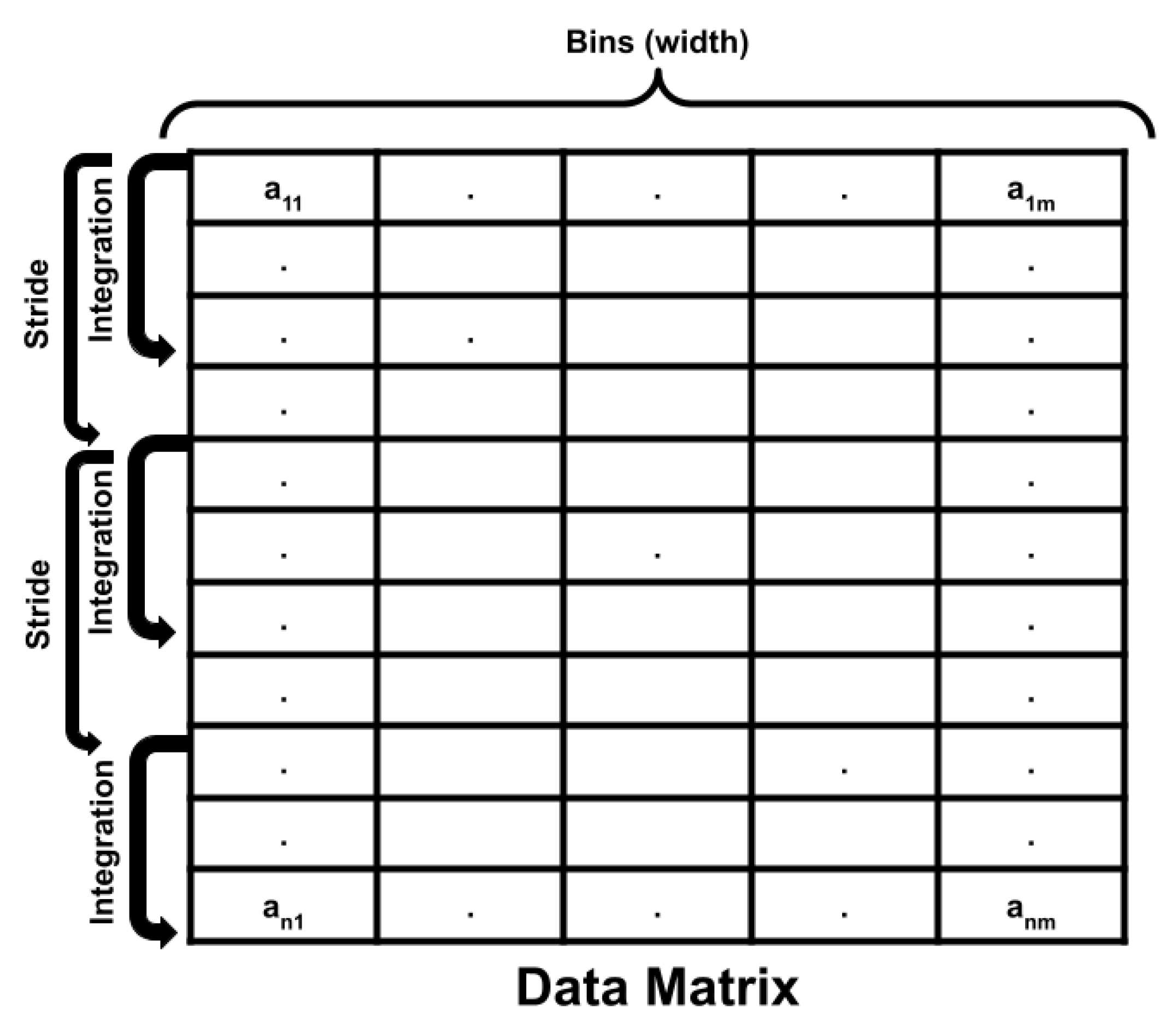
First, a model is constructed to identify anomalous measurements from the temporally continuous radiation data stream. This model ingests energy-independent count rates for each minute of measurement. That is, the one-second, 1000-bin measurements are integrated for all energies and every second in a one-minute window. This results in a "gross" count rate that is a raw measure of the number of gamma emissions counted by the NaI detector in that period. All of this data pre-processing occurs in RadClass—the software suite developed for this analysis—as shown in Figure 5.

A method of hypothesis testing is employed that was originally used in counting statistics [17]. Given two measurements, $x_1$ and $x_2$ (in this case, one-minute gross count-rates), taken at times $t_1$ and $t_2$, respectively, it is expected that they are each sampled from some statistical distribution. In the case of radiation counting statistics,

$$\begin{array}{cc}\hfill & x_1\sim \mathrm{Poisson}\left({\mu }_1\right)\hfill \\ \hfill & x_2\sim \mathrm{Poisson}\left({\mu }_2\right),\hfill \end{array}$$

(4)

where ${\mu }_1$ and ${\mu }_2$ are the expected values of the Poisson distribution. If the magnitudes of $x_1$ and $x_2$ are approximately equivalent, then they likely come from the same distribution. For example, if that distribution is the background, then they can both confidently be labeled as coming from the background. However, if their magnitudes are appreciably different, then they should be labeled as anomalous, i.e., from different statistical distributions:

$$\begin{array}{cc}\hfill & H_0:{\mu }_1={\mu }_2\hfill \\ \hfill & H_1:{\mu }_1\ne {\mu }_2.\hfill \end{array}$$

(5)

This anomalous behavior could be from a nuclear material transfer or from any other kind of radiation event off-normal for the defined background distribution. Anomalies depend on the rate of change between $t_1$ and $t_2$ to be recognized as having sufficiently varying magnitudes. The expected values, ${\mu }_1$ and ${\mu }_2$, are typically not measurable without enough unbiased samples. Suppose $H_0$ is true, then a mathematical translation can be made:

$$\begin{array}{cc}\hfill & n=x_1+x_2\hfill \\ \hfill & \mu ={\mu }_1+{\mu }_2\hfill \\ \hfill & p=\frac{{\mu }_1}{{\mu }_2+{\mu }_2}=\frac{1}{2}.\hfill \end{array}$$

(6)

Therefore, comparing one measurement, $x_1$, with the sum of both measurements, n, behaves like a binomial distribution

$$x_1\mid x_1+x_2\sim \mathrm{Binomial}(x_1,n,\frac{1}{2}).$$

(7)

If $H_1$ is true, then the binomial test above will fail to some significance level. This binomial test can be completed using MINOS data and identifies anomalous measurements in a temporal dataset. Each consecutive pair of measurements is tested, a p value is computed, and the null hypothesis is either accepted or rejected to some significance level. For a specified significance level, certain amounts of deviation are tolerated beyond which the null hypothesis is rejected, and an anomaly is identified. This significance level threshold acts as a hyperparameter and must be set via optimization using a ground-truth reference.

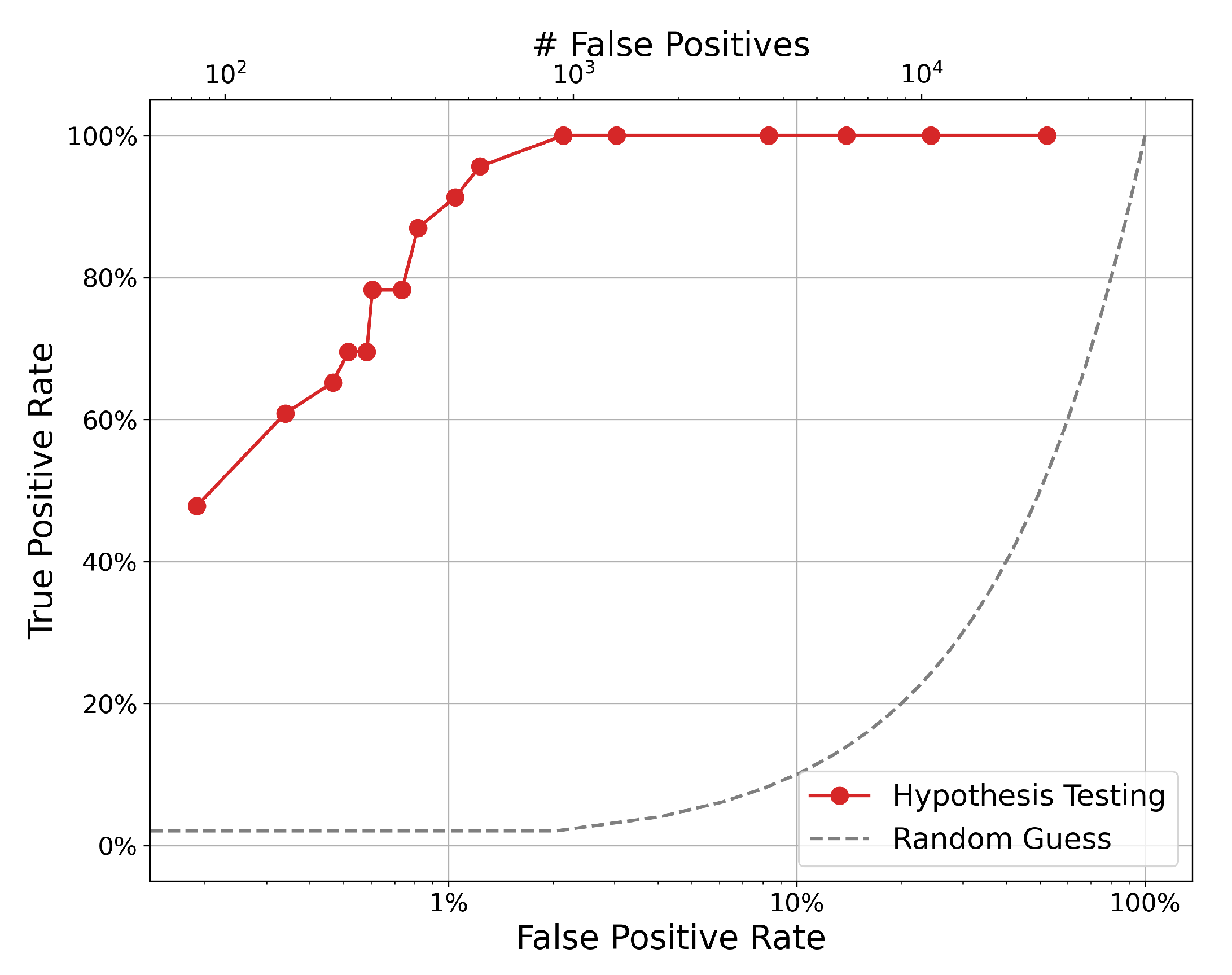
Using one node, one month of data (approximately 43,200 measurements) and ground truth for transfers, a receiver operating characteristic (ROC) curve can be generated (see Figure 6). Here, a positive is defined as a prediction of a transfer event, and a negative is a prediction of some other anomalous event. First, the number of correct positive classifications can be expressed as the true positive rate: $\mathrm{Recall}=TPR=\frac{TP}{TP+FN}$. The rate of positive misclassifications can be expressed as the false positive rate: $FPR=\frac{FP}{TN+FP}$. True positives are defined here as an anomalous measurement taken within 20 min of the timestamp for the event in ground truth or, absent a specific ground-truth timestamp, one anomalous measurement in a given day with a recorded transfer. This accounts for transportation and detector efficiencies that delay nuclear material transfers from being registered in a detector response for some time after the event may be recorded in ground truth.

Note that the ROC curve sweeps over several values for significance level. An ideal significance level is one that maximizes true positives while minimizing false positives. However, true positives (i.e., material transfers) are rare in the dataset compared to the measurement frequency. This leads to an imbalance in the number of true positives and true negatives. That is, a percentage increase in the $FPR$ is a larger increase in magnitude of false positives than a comparable percentage increase in the $TPR$.

For example, the tenth point (a significance level of $0.001$) registers 22 out of 23 true positives ($TPR=95.7\%$) with a $FPR$ of only 1.2%. In gross terms, this false-positive rate corresponds to 540 one-minute false-positive measurements. The next significance level of $0.005$ captures the last true positive at the cost of an additional 397 false positives ($TPR=100\%$, $FPR=2.1\%$). This imbalance must be considered in choosing a strict value for training and testing the models below.

The p value used for the analysis below is ${10}^{-20}$, which is the strictest value tested with a true positive rate of only about 40% but is also the smallest false positive rate tested. Future experiments can loosen this restriction by using a larger significance level that increases the number of true positives and false positives and thereby furthers the need for event discrimination. The overall magnitude of false positives is very large in part because of noisy ground-truth labeling. A small significance level is chosen to avoid confounding the machine learning models tested below with a large number of false positives, especially since the ground truth will not be used moving forward. This further emphasizes the need to carefully discriminate between SNM transfers and other anomalous measurements in any downstream analyses.

3.5. Labeling Heuristic

In evaluating the predictive accuracy of the machine learning models described below, three data subsets must be created: labeled training data, unlabeled training data, and labeled testing data. First, five months of energy-independent (gross count-rate) data from six different MINOS nodes are passed through the hypothesis-testing algorithm with a temporal integration time of one-minute. This provides a collection of spectra for timestamps at which the gross count rate was deemed anomalous (i.e., the null hypothesis was rejected). For this and all downstream tasks, the background is removed from the anomalous spectrum by estimation. It is assumed that for each event, a spectrum taken 20 min prior would constitute a typical background distribution absent any radiation events. This is subtracted from the event spectrum, resulting in a feature vector that notionally consists of only energy-dependent counts associated with the anomalous event (called the difference spectrum, illustrated in Figure 3).

Rather than using the ground truth to apply labels to the data, a labeling heuristic applies an automated "guess" that serves as a noisy label (i.e., with nonzero labeling error) for each sample. That guess could be a material transfer, ⁴¹Ar event, Radon washout, or other anomalous behavior. The labeling heuristic uses Scikit-learn’s find_peaks method to estimate the most prominent peaks in each spectrum. If one of those peaks appears within an energy range where signatures resulting from shielded radiological material transfers would be expected, and that peak is sufficiently prominent, the labeling heuristic assigns a material transfer guess to that sample. If not, a different label may apply. If none of the peaks are prominent enough to make a definitive guess, the spectrum is not labeled, and the sample is removed from the collection of anomalies.

In this way, the labeling heuristic applies a noisy label prediction to samples without relying on ground-truth information. This heuristic itself is not a sufficient model for discriminating between SNM transfers and other anomalous events because its accuracy is limited by an intrinsic error rate related to noisy labeling. The labeling heuristic is still better than random guessing because it applies limited domain knowledge related to expected behavior from material transfers and the detector response from MINOS. Therefore, these labels can appropriately be used for training and testing machine learning models because the uncertainty associated with noisy labeling is propagated to each model and is thus invariant when comparing models to each other. Any uncertainty associated with the labeling heuristic will be propagated to each model trained and tested on the resulting labels. Therefore, MINOS data can be used to train and compare ML models, avoiding reliance on ground truth for preparing training data.

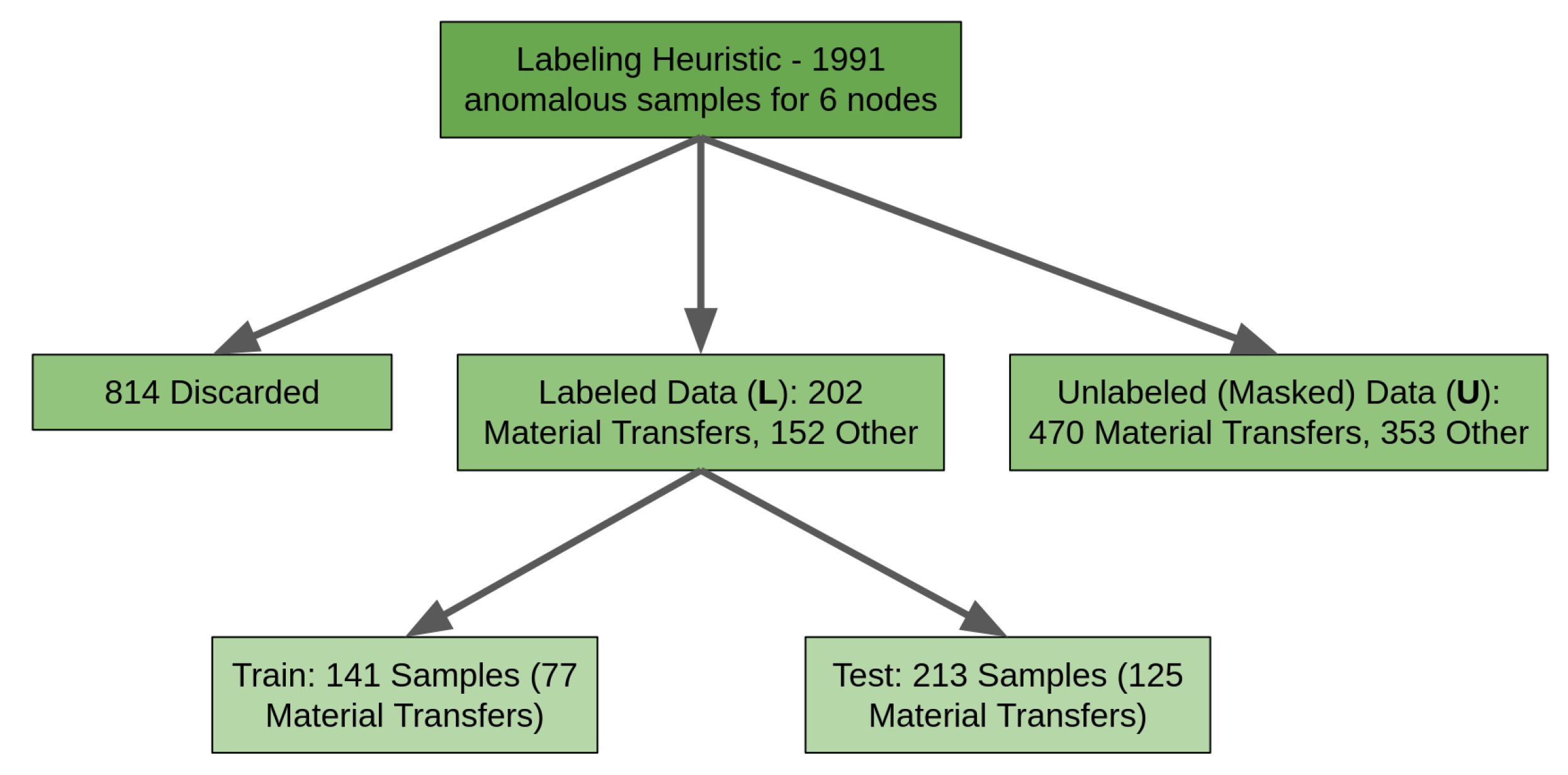
The labels are organized for binary classification: material transfer or "other" anomalous measurement. The labeled corpus is then randomly split into small subsets that approximately maintain the binary class population ratio. The remaining majority are passed (as unlabeled data) with their label masked from any models or evaluation techniques. This simulates the real-world behavior of costly labeling in which it may be difficult to label a large amount of data, but a smaller amount is still feasible. Labeling these unlabeled data was not necessary (since the label was not stored) but it ensured that the labeled and unlabeled subsets had similar distributions of classes. The heuristic is summarized in Figure 7.

4. Machine Learning Models

4.1. Supervised

Logistic Regression

Logistic regression serves as the baseline supervised model to be compared with semi-supervised machine learning. This model minimizes a loss function on labeled data:

$$\underset{w,c}{min}\frac{1}{2}{w}^{T}w+C\sum _{i=1}^{n}log(exp(-y_i(x_i^{T}w+c))+1).$$

(8)

where w is a weight vector that predicts a label from some sample $x_i$ with a bias term c. The model minimizes the disagreement between a predicted label $x_i^{T}w$ and the actual label $y_i$ while minimizing the magnitude of weight values in w (L2 regularization). Logistic regression requires a fully labeled training corpus and cannot utilize unlabeled data in this form. Therefore, this model only trains on $\mathit{L}$. This can be problematic in a costly labeling regime where labeled data are less voluminous.

4.2. Semi-Supervised

4.2.1. Co-Training with Logistic Regression

This first semi-supervised machine learning model extends the supervised logistic regression model above to handle unlabeled data. Two supervised logistic regression models are trained in tandem, passing information gained between each other, called co-training [18]. The logic is described in Algorithm 1. Each model learns some information from its training corpus so that it can predict an unlabeled sample, and it trades this information with its partner model. Ideally, the two models will converge to some increased level of accuracy because of shared information learned from each other (observed in Figure 8).

Algorithm 1 Co-training

Given: $\mathit{L}$ and $\mathit{U}$, split $\mathit{L}$ between two logistic regression models ($h_1$ and $h_2$) while $\mathrm{len}\left(\mathit{U}\right)>0$ do    Train $h_1$ and $h_2$ on their portions of labeled data, ${\mathit{L}}_{\mathbf{1}}$ and ${\mathit{L}}_{\mathbf{2}}$    Have $h_1$ predict $u_1$ and $h_2$ predict $u_2$, $\parallel u_1+u_2\parallel \le \parallel U\parallel /2$ sampled from $\mathit{U}$.    Include $u_1$ in ${\mathit{L}}_{\mathbf{2}}$ and $u_2$ in ${\mathit{L}}_{\mathbf{1}}$ with their predicted labels; remove from $\mathit{U}$.    Repeat training with this newly labeled unlabeled samples end while Evaluate on test set

4.2.2. Label Propagation

Label propagation [19] is a transductive approach that acts like a semi-unsupervised model. This algorithm propagates labels from labeled data, $\mathit{L}$, to unlabeled data, $\mathit{U}$. Propagation is accomplished by comparing distances between data samples, whatever that notion of distance might be. First, data are arranged as a fully connected graph with edge weights defined by some kernel. In this experiment, a radial basis function (RBF) is used:

$$w_{i,j}=exp(-\frac{\left|\right|x_i-x_j{\left|\right|}^2}{{\sigma }^2}).$$

(9)

where $\sigma$ is essentially the standard deviation in the dataset or can be learned as a hyperparameter. This is used to create a transition matrix, T, which updates the label matrix, Y, with dimensions $\left(\right|\mathit{L}|+|\mathit{U}\left|\right)\times C$ where C is the number of classes ($C=2$ for binary classification). Each row is the probability of that sample being labeled with each respective class. If, for example, a row was associated with a labeled instance for the first class, its row would be $[1.0,0.0]$. TO reiterate, propagate using $Y\leftarrow TY$, normalize row-wise, and clamp any labeled rows to conform with their labeled classification instances. Afterward, an argmax can be applied to classify each row according to the most probable label.

This is guaranteed to converge to a unique solution [19]. Therefore, there is no training step per se if sufficient propagation iterations have occurred. This is also the only semi-supervised machine learning algorithm used in this work that is readily available in Scikit-learn. Only two other SSML models have been implemented: label spreading and a self-training classifier.

4.2.3. Convolutional Neural Network

An artificial neural network (ANN) is a form of machine learning model that is designed around networks of connected neurons consisting of unique activation functions that train for predictive classification by learning patterns in labeled data. These networks can be large or deep, which allows them to be flexible in pattern recognition but which requires copious amounts of data for training. In principle, CNNs are designed to pass filters over data and to convolve data structures for more robust feature representation. This operation is also shift invariant, making it effective for nonlinear patterns.

Shadow [20] is a Python package with loss functions that can be applied to various neural networks implemented in PyTorch. Originally designed for seismological data, these loss functions are data agnostic and include semi-supervised functions for processing unlabeled data in a neural network. Given some model, $f_{\theta }$, the loss function is divided into two portions:

$$\mathcal{L}(f_{\theta }\left(x_l\right),y_l)+\alpha g(f_{\theta },x).$$

(10)

In this case, $f_{\theta }$ is a CNN and can predict a classification label for an instance, $x_l$, and $\mathcal{L}$ compares it to the actual label, $y_l$, where labeled data exist. The model can also be passed to a consistency-enforcing function, $g(·)$, alongside any data instance (labeled or unlabeled) and penalizes differences given some perturbation. The consistency-enforcing function is weighted in the overall loss function by a hyperparameter, $\alpha$. The loss function, $g(·)$, used here is exponential averaging adversarial training (EAAT) [20]

$$g(f_{\theta },x)=d(f_{\theta }(x+r_{\mathrm{adv}}),f_{\theta }^{{}^{\prime }}\left(x\right)),$$

(11)

where $d(·)$ is a distance metric that describes the difference between its two inputs: the exponential moving average teacher, $f_{\theta }^{{}^{\prime }}$, and its student, $f_{\theta }$. Here, a small perturbation, $r_{\mathrm{adv}}$, is added to the data. Utilizing the cluster assumption, a sufficiently small perturbation should not affect the predicted label since samples close together in state space should have similar classifications. The EAAT algorithm combines virtual adversarial training (VAT) with mean teacher (MT). Virtual adversarial training chooses perturbations that produce the largest change in model output to enforce regularization. Mean teacher sets model weights using an exponential moving average, which is shown to produce more stable predictions.

In practice, both labeled and unlabeled data are processed by a CNN, optimized using stochastic gradient descent (SGD) with a cross-entropy loss function, and employs the cluster assumption to better probe the decision boundary for classification. The initial neural network architecture for this model is based on an example structure for handling MNIST data [21], which comprise a collection of 2D images of handwritten digits. Instead of accepting 2D image inputs, the model here accepts 1D spectra. Figure 9 shows the initial CNN architecture prior to hyperparameter optimization. As the loss function is minimized, the model is optimized by maximizing the classification of labeled instances and enforcing consistency among unlabeled data (see Figure 10). The loss decreases over the training period. However, the variability—or noise—over epochs shows that certain instabilities may prevent further loss minimization or outright convergence.

5. Results

Hyperparameter optimization was implemented using the Hyperopt [22] software package. This method uses Bayesian inference to explore the hyperparameter state space and to find the model parameters that maximize classification accuracy. Hyperparameters are chosen in a direction of expected accuracy increase. The loss function for optimization is the error rate, which Hyperopt attempts to minimize. Different hyperparameters are chosen over 100 tuning epochs. The resulting performance ranges are shown in

Table 1. Hyperparameter optimization balanced accuracy results.

Model	Worst (%)	Best (%)
Logistic Regression	63.9	67.7
Co-training	56.1	71.8
Label Propagation	55.1	77.1
Shadow EAAT	48.4	70.9

. Local minima are possible for more complex models, but convergence typically occurs well before 100 tuning epochs.

The following metrics for binary classification—relating correctly classified instances, true positives ($TP$) and true negatives ($TN$), to misclassifications, false positives ($FP$) and negatives ($FP$)—are used in evaluating a model’s performance:

$$\begin{array}{cc}\hfill \mathrm{Accuracy}& =\frac{TP+TN}{TP+FP+TN+FN}\hfill \\ \hfill \mathrm{Balanced}\mathrm{Accuracy}& =\frac{1}{2}(\frac{TP}{TP+FN}+\frac{TN}{TN+FP})\hfill \\ \hfill \mathrm{Precision}& =\frac{TP}{TP+FP}\hfill \\ \hfill \mathrm{Recall}& =\frac{TP}{TP+FN}.\hfill \end{array}$$

(12)

Balanced accuracy (balanced for different class populations) will be used as a concise measure for comparing models. Several feature vector normalization options were also tested to maximize accuracy. Label propagation benefited from input features that were not normalized, since it measures distances between samples. Therefore, any notional distance exhibited by data samples would be affected by normalization, reducing label propagation’s performance. Shadow significantly benefited from normalization against the distribution’s mean and standard deviation, since the neural network’s loss function is sensitive to large feature magnitudes. K-fold cross-validation was studied on logistic regression and co-training to ensure that there was no accuracy biasing because of random train–test splits. No appreciable difference was noted from different random splits.

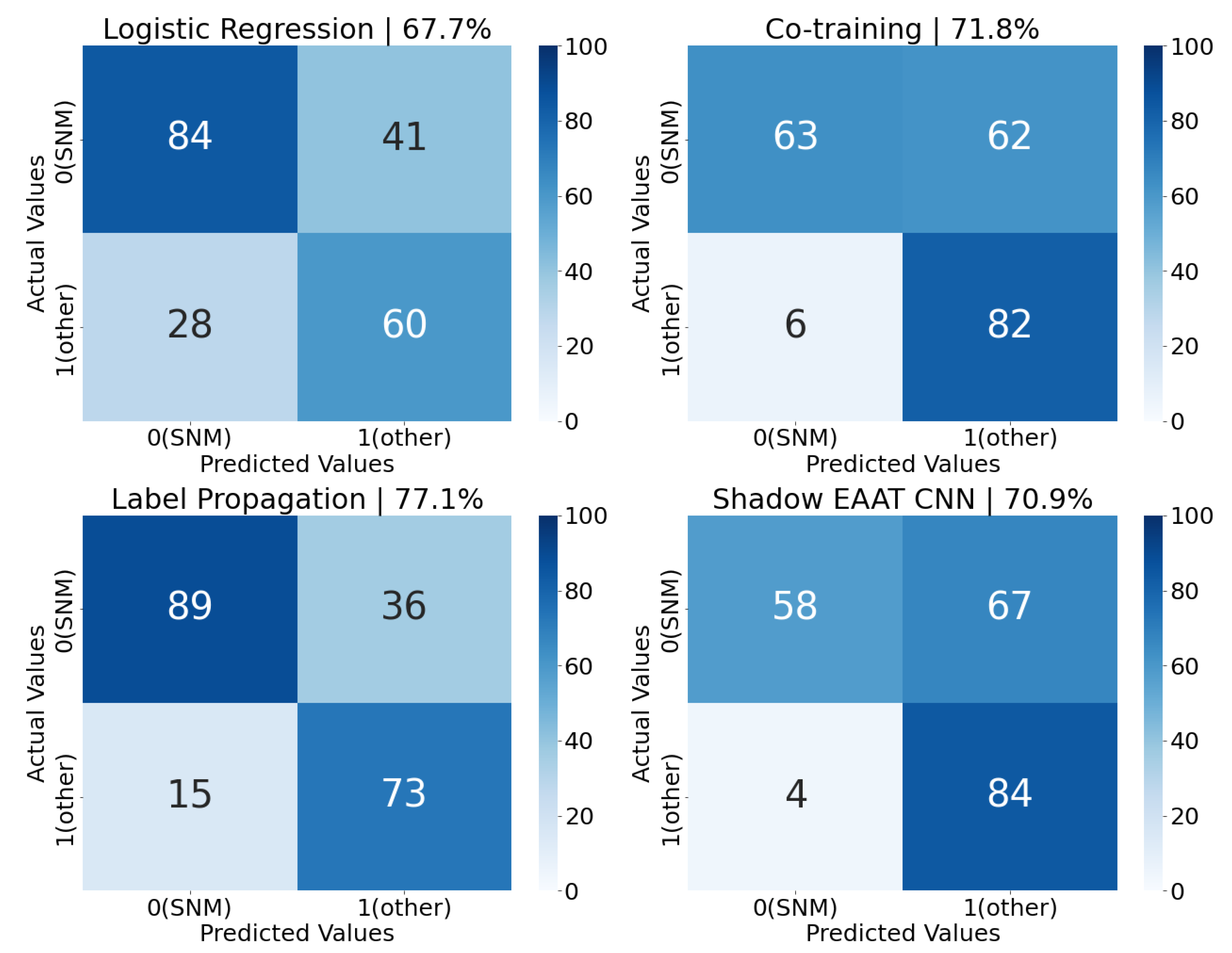
Confusion matrices for each model’s best balanced accuracy score (from Table 1) can be seen in Figure 11. The models, in order of increasing maximum balanced accuracy achieved, are: logistic regression, Shadow, co-training, and label propagation. None of the models tested predicted more false positives than false negatives, leading each to have a higher precision than recall. Co-training and Shadow, despite having comparable balanced accuracy scores, have exceptionally low recall (and very high precision) due to numerous false negatives, and only a handful of false positives. False positives are arguably less impactful than false negatives (i.e., recall is more important than precision) since detecting all instances of SNM transfers is the desired objective. In practice, the level of tolerance for false positives and false negatives is influenced by the needs of an end-user. A policy could be designed that weights these factors in model optimization or guides the deployment choice from a selection of trained models.

Several possible explanations exist for each model’s accuracy. Logistic regression performs the worst of all four methods, suggesting that it is not generalizable to the test dataset. That is, this model has relatively simple complexity but is still capable of learning a decision boundary within the limited labeled training dataset. A more complex supervised model, such as a multilayer perceptron (MLP), could possibly generalize, but these methods are typically data hungry. This illustrates the challenge of using supervised models in this regime because a large, labeled data corpus is required to achieve high performance, but collecting such a dataset is costly (perhaps infeasible).

Co-training achieves a higher balanced accuracy because it utilizes previously unused unlabeled data. However, the increase in accuracy is likely limited by the structure of the data algorithm used. The authors of this method state that the two sets of labeled data, ${\mathit{L}}_{\mathbf{1}}$ and ${\mathit{L}}_{\mathbf{2}}$, must exhibit conditional independence. That is, $X_1\perp X_2\mid Y$, i.e., each subset contains predictive information for the classification but not for its counterpart. This is enforced so that each model learns different information to share. If ${\mathit{L}}_{\mathbf{1}}$ and ${\mathit{L}}_{\mathbf{2}}$ do not exhibit conditional independence, convergence to a higher accuracy is not guaranteed.

The data passed here are not necessarily conditionally independent. Only radiation data are used, and the measurements of all nodes are combined into one corpus. Two measurements from the same detector, and even for the same event, could be present in the training data for both models, breaking independence. Any increase in performance from training could be the result of information passed between models that is from different detectors and events. Co-training’s accuracy could be increased by enforcing conditional independence and by carefully separating detectors between models. A more powerful implementation would utilize data fusion, a natural extension of MINOS. For example, one model could be trained on seismo-acoustic data, and one model could be trained on radiation measurements, both of which are coincident on SNM transfers but conditionally independent of each other.

Label propagation achieves the highest recall among the four models used (with the largest number of true positives classified). This is likely because label propagation is the only model to consider the geometric or distance relationship between data points, thus indicating that pattern information could be embedded in the data manifold. A manifold pattern also suggests some feature importance, or low-dimensional representation, which leads to eventual classifications. This agrees with physical intuition that radiation signatures are energy-dependent and should be unique between transfers of shielded radiological material and other types of radiation events.

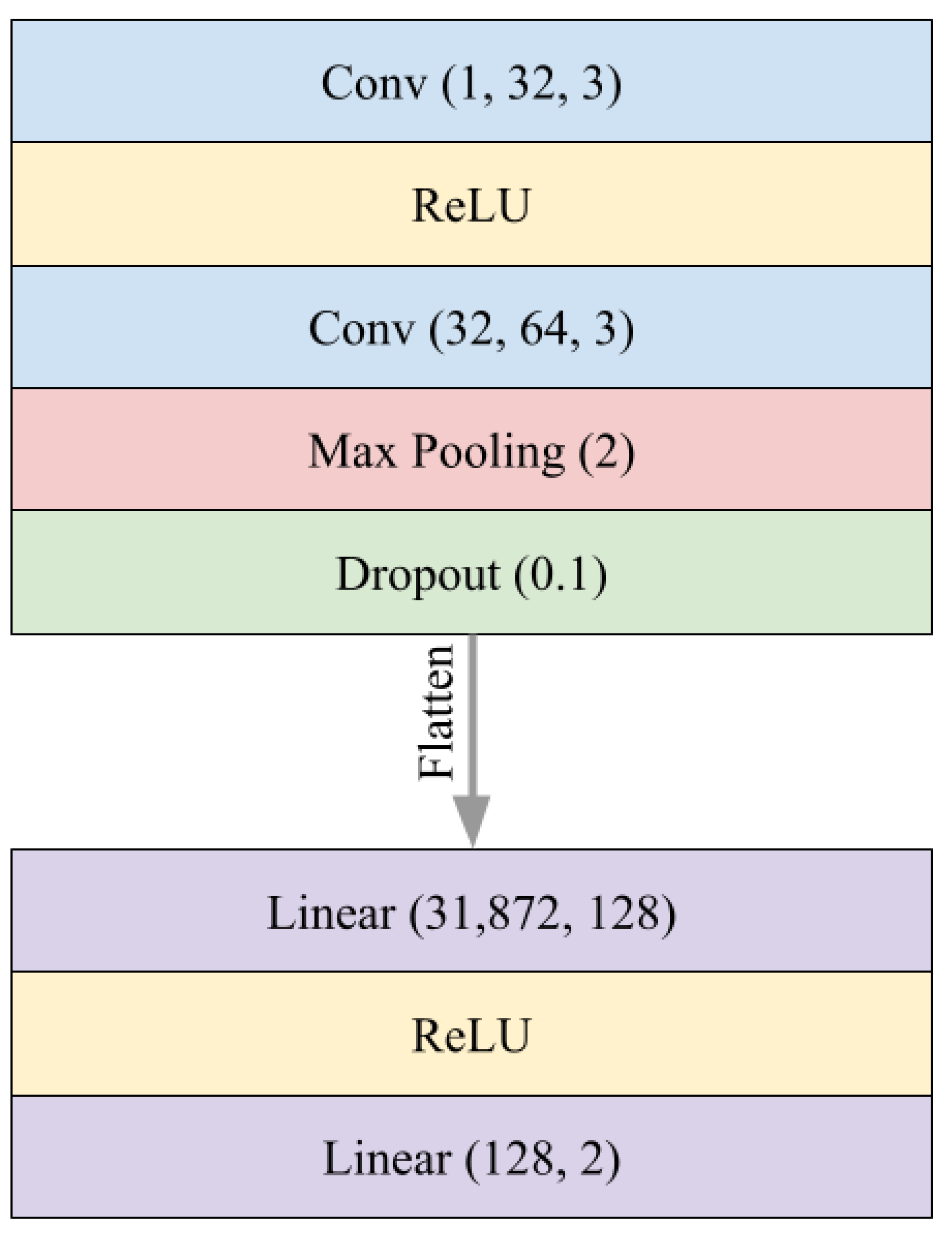
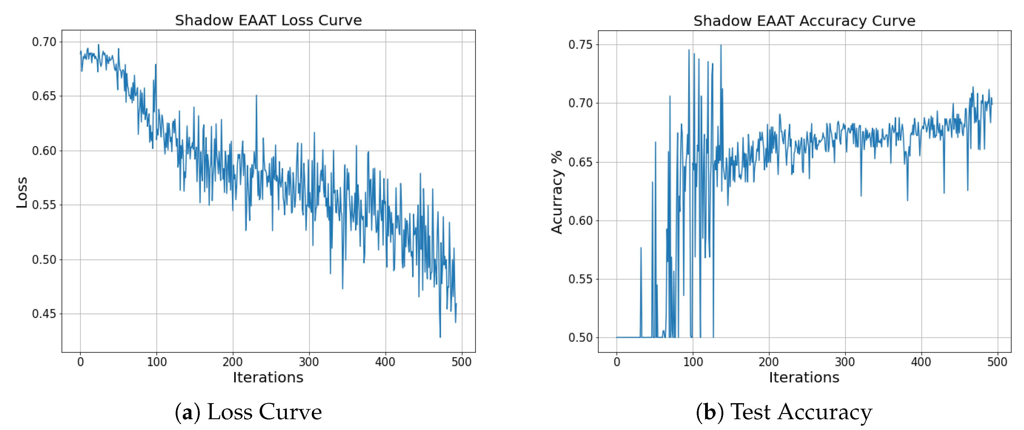
Finally, Shadow’s performance was surprisingly the lowest among the semi-supervised models. Shadow’s CNN has many hyperparameters that can be further optimized, including the architecture of the network itself. The MNIST structure used here might not lend itself to spectral data. Rather, a network architecture such as those used for frequency/audio data could be used. The loss function may be too difficult to minimize for high-variance data such as radiation spectra. Training indicated that Shadow can optimize to many local minima in its state space. Different loss functions could be applied, including different semi-supervised functions, that may train with more stability or converge to an optimal decision boundary. Overall, a CNN still requires significant amounts of data to train an accurate classifier. Despite the inclusion of unlabeled data, more labeled (and unlabeled) data could be required to find an effective decision boundary.

6. Conclusions

Nuclear material transfer detection methods that reduce computing and domain costs while maintaining detection performance can be an important component toward advancing nuclear nonproliferation. Models using SSML can alleviate the high cost of labeling radiation samples while still utilizing otherwise unused unlabeled data to build robust ML models for the detection of SNM transfers. The work presented here applied an anomaly-detection algorithm to analyze radiation data collected at the MINOS testbed and to distinguish radiation events from background. A labeling heuristic was designed to study the effects of noisy labeling on training data to reduce the reliance on ground truth or on unreliable prior knowledge. All the semi-supervised models tested performed with higher accuracy than a supervised logistic regression benchmark, indicating that it is possible to utilize labeled and unlabeled data in SSML models for detecting and characterizing SNM transfers. The increased accuracy of SSML models suggests that there is still valuable classification information about the data distribution present in unlabeled data. This warrants more detailed work to study the effects of learning on unlabeled data using more advanced systems of SSML techniques.

References

1. Office of General Council, U.S. Nuclear Regulatory Commission. Nuclear Regulatory Legislation, 112th Congress; 2nd Session; Technical Report 10; U.S. Nuclear Regulatory Commission: Washington, DC, USA, 2013.
2. IAEA. Annual Report for 2020; Technical Report; International Atomic Energy Agency: Vienna, Austria, 2020.
3. Ma, J.; Jiang, J. Semisupervised classification for fault diagnosis in nuclear power plants. Nucl. Eng. Technol. 2015, 47, 176–186. [Google Scholar] [CrossRef] [Green Version]
4. Pinciroli, L.; Baraldi, P.; Shokry, A.; Zio, E.; Seraoui, R.; Mai, C. A semi-supervised method for the characterization of degradation of nuclear power plants steam generators. Prog. Nucl. Energy 2021, 131, 103580. [Google Scholar] [CrossRef]
5. Sun, L.; Zhao, C.; Yan, Z.; Liu, P.; Duckett, T.; Stolkin, R. A Novel Weakly-Supervised Approach for RGB-D-Based Nuclear Waste Object Detection. IEEE Sens. J. 2019, 19, 3487–3500. [Google Scholar] [CrossRef] [Green Version]
6. Moshkbar-Bakhshayesh, K.; Ghofrani, M.B. Combining Supervised and Semi-Supervised Learning in the Design of a New Identifier for NPPs Transients. IEEE Trans. Nucl. Sci. 2016, 63, 1882–1888. [Google Scholar] [CrossRef]
7. Moshkbar-Bakhshayesh, K.; Mohtashami, S. Classification of NPPs transients using change of representation technique: A hybrid of unsupervised MSOM and supervised SVM. Prog. Nucl. Energy 2019, 117, 103100. [Google Scholar] [CrossRef]
8. Nicholson, A.D.; Archer, D.E.; Garishvili, I.; Stewart, I.R.; Willis, M.J. Characterization of gamma-ray background outside of the High Flux Isotope Reactor. J. Radioanal. Nucl. Chem. 2018, 318, 361–367. [Google Scholar] [CrossRef]
9. Dayman, K.; Hite, J.; Hunley, R.; Rao, N.S.V.; Geulich, C.; Willis, M.; Ghawaly, J.; Archer, D.; Johnson, J. Tracking Material Transfers at a Nuclear Facility with Physics-Informed Machine Learning and Data Fusion. In Proceedings of the INMM & ESARDA Joint Annual Meeting, Virtual, 30 August–1 September 2021. [Google Scholar]
10. Shalev-Shwartz, S.; Ben-David, S. Understanding Machine Learning: From Theory to Algorithms; Cambridge University Press: Cambridge, UK, 2014. [Google Scholar]
11. Russell, S.; Norvig, P. Artificial Intelligence: A Modern Approach, 4th ed.; Prentice Hall: Hoboken, NJ, USA, 2020. [Google Scholar]
12. Devroye, L.; Györfi, L.; Lugosi, G. A Probabilistic Theory of Pattern Recognition; Stochastic Modelling and Applied Probability; Springer: Berlin/Heidelberg, Germany, 1996; Volume 31. [Google Scholar] [CrossRef]
13. Chapelle, O.; Schölkopf, B.; Zien, A. Semi-Supervised Learning; The MIT Press: Cambridge, MA, USA, 2006. [Google Scholar]
14. Lu, T. (Tian). Fundamental Limitations of Semi-Supervised Learning. Master’s Thesis, University of Waterloo, Waterloo, ON, Canada, 2009. [Google Scholar]
15. Singh, A.; Nowak, R.; Zhu, J. Unlabeled data: Now it helps, now it doesn’t. In Proceedings of the Advances in Neural Information Processing Systems, Vancouver, BC, Canada, 8–11 December 2008; Volume 21. [Google Scholar]
16. van Engelen, J.E.; Hoos, H.H. A survey on semi-supervised learning. Mach. Learn. 2020, 109, 373–440. [Google Scholar] [CrossRef] [Green Version]
17. Przyborowski, J.; Wilenski, H. Homogeneity of Results in Testing Samples from Poisson Series: With an Application to Testing Clover Seed for Dodder. Biometrika 1940, 31, 313–323. [Google Scholar] [CrossRef]
18. Blum, A.; Mitchell, T. Combining Labeled and Unlabeled Data with Co-Training. In Proceedings of the Eleventh Annual Conference on Computational Learning Theory, Madison, WI, USA, 24–26 July 1998; pp. 92–100. [Google Scholar] [CrossRef]
19. Zhu, X.; Ghahramani, Z. Learning from Labeled and Unlabeled Data with Label Propagation; Technical Report; Carnegie Mellon University: Pittsburgh, PA, USA, 2003. [Google Scholar]
20. Linville, L.; Anderson, D.; Michalenko, J.; Galasso, J.; Draelos, T. Semisupervised Learning for Seismic Monitoring Applications. Seismol. Res. Lett. 2020, 92, 388–395. [Google Scholar] [CrossRef]
21. Shadow Documentation MNIST Example. Available online: https://shadow-ssml.readthedocs.io/en/latest/examples/mnist_example.html (accessed on 3 July 2023).
22. Bergstra, J.; Yamins, D.; Cox, D. Making a Science of Model Search: Hyperparameter Optimization in Hundreds of Dimensions for Vision Architectures. In Proceedings of the 30th International Conference on Machine Learning, ICML 2013, Atlanta, GA, USA, 16–21 June 2013; Volume 28, pp. 115–123. [Google Scholar]
Figure 2. Here is an example of a radiation spectrum taken from MINOS. Note several spectral features, including photopeaks associated with background radiation (labeled).
Jne 04 00032 g002
Figure 3. A radiation spectrum taken when material was present (orange). Note the high count-rate and low energy distribution associated with a transfer. In an attempt to accentuate this feature, an approximated background distribution (gray) is subtracted from the event spectrum to obtain a difference (blue) only associated with the anomalous features.
Jne 04 00032 g003
Figure 4. One-minute gamma radiation spectrum measurements collected over one month, collected into one plot. Here, each vertical slice (energy bin) is a normalized frequency histogram. Color indicates the frequency at which the count-rate associated with each energy was measured at that specific magnitude.
Jne 04 00032 g004
Figure 5. RadClass expects a standardized data format that can be abstracted to an n by m matrix with n temporal instances and m bins of data. For MINOS radiation measurements, this would be 1-second temporal instances and 1000 energy bins. For example, one month would be approximately a 43,200 × 1000 matrix. Given an integration time, RadClass will collapse and integrate a set of rows for every column. If the integration time is 60 seconds, every 60 rows will be integrated column-wise. An optional stride parameter could be defined to overlap or skip rows for integration.
Jne 04 00032 g005
Figure 6. ROC for one node and one month of data using energy-independent, 1-minute count rates. Individual red points on the curve indicate different significance levels, which vary how strictly to enforce the measurement equivalence. As the significance level becomes larger, more and more null hypotheses are rejected, capturing more true and false positives. The gray dotted line indicates a 50–50 ratio, equivalent to an algorithm that makes a random guess for classification.
Jne 04 00032 g006
Figure 7. The breakdown for sample splits between labeled training, labeled testing, and unlabeled data from the labeling heuristic. Note that using 5 months and 6 nodes worth of data results in 1991 anomalous measurements, where 814 are discarded since their label could not be resolved by the heuristic, and the rest are divided proportionally into train, test, and unlabeled subsets.
Jne 04 00032 g007
Figure 8. The test accuracy for each co-training model as trained using Algorithm 1. Test accuracy is defined as the percentage of correctly classified samples in a test set not used in training the models (refer to Equation (12)). Ideally, both models would converge to a higher accuracy, indicating that information passed between models was helpful for learning and pattern recognition. A marginal increase is observed here.
Jne 04 00032 g008
Figure 9. The base (prior to hyperparameter optimization) architecture for the CNN used by Shadow EAAT. This consists of two convolution layers with max pooling and dropout, resulting in a representation that is passed to linear, connected layers ending in a binary classification prediction. This was offered as an example architecture for analyzing MNIST data by Shadow [21], adjusted for accepting 1D spectra rather than 2D images.
Jne 04 00032 g009
Figure 10. The results of training for the best Shadow model found via hyperparameter optimization. (a) The results of the loss function optimized during training: cross-entropy loss with EAAT optimized using SGD. (b) Accuracy on test data for every epoch. Accuracy notionally increases as the model is optimized, with early stopping resulting in a test accuracy greater than 70%.
Jne 04 00032 g010
Figure 11. Confusion matrices on test datasets for each machine learning model. Note that the scores above for each confusion matrix are its respective balanced accuracy. SNM, class label 0, represents a positive, and other, class label 1, represents a negative.
Jne 04 00032 g011