Multi-Abnormality Attention Diagnosis Model Using One-vs-Rest Classifier in a Nuclear Power Plant

Abstract

Multi-abnormal events, referring to the simultaneous occurrence of multiple single abnormal events in a nuclear power plant, have not been subject to consideration because multi-abnormal events are extremely unlikely to occur and indeed have not yet occurred. Such events, though, would be more challenging to diagnose than general single abnormal events, exacerbating the human error issue. This study introduces an efficient abnormality diagnosis model that covers multi-abnormality diagnosis using a one-vs-rest classifier and compares it with other artificial intelligence models. The multi-abnormality attention diagnosis model deals with multi-label classification problems, for which two methods are proposed. First, a method to effectively cluster single and multi-abnormal events is introduced based on the predicted probability distribution of each abnormal event. Second, a one-vs-rest classifier with high accuracy is employed as an efficient way to obtain knowledge on which particular multi-abnormal events are the most difficult to diagnose and therefore require the most attention to improve the multi-label classification performance in terms of data usage. The developed multi-abnormality attention diagnosis model can reduce human errors of operators due to excessive information and limited time when unexpected multi-abnormal events occur by providing diagnosis results as part of an operator support system.

1. Introduction

The operation modes of general Korean pressurized water reactors (PWRs) are classified into six categories. Mode 6 corresponds to refueling, while modes 5 to 1, respectively, cycle between cold shutdown, hot shutdown, hot standby, startup, and power operation. During power operation (mode 1), the nuclear power plant (NPP) generates electricity following three sorts of operating procedures: general operating procedures in normal conditions, abnormal operating procedures (AOPs) in abnormal events, and emergency operating procedures in emergency situations. In an abnormal transient, the operators must find the appropriate AOP for the situation based on the information from thousands of dynamic plant parameters within a limited time and take action. Depending on the measures taken by the operators, the NPP may return to a normal condition or enter an emergency situation accompanied by a reactor shutdown.

In the case of the Korean Advanced Power Reactor 1400 (APR-1400), there are 82 AOPs with 224 sub-procedures. When an abnormal event occurs, the operators recognize the transition into the abnormality through alarms in the main control room (MCR). Operators then must correctly diagnose the abnormal event according to one of the 224 sub-procedures of the AOPs while under hundreds of indicators and thousands of power plant parameters [1]. With limited time, these large amounts of plant parameters and AOPs can burden operators, potentially leading to a misdiagnosis and worsened situations such as a reactor trip.

The safety systems of NPPs have undergone extensive development after facing unexpected accidents. For instance, research on human reliability has been actively conducted since the Three Mile Island accident, and countermeasures to the extended loss of alternating current power have been discussed after the Fukushima Daiichi accident [2,3]. According to Korea’s operational performance information system for nuclear power plants, unexpected shutdowns of reactors due to human error amount to about 20 percent of all shutdowns, and to cope with human error, some studies have been conducted to support MCR operators in abnormal transients using artificial intelligence (AI) based on improved computing resources [4,5]. Previous studies mainly focused on diagnosing single abnormal events in the role of operator support systems with neural networks. Multi-abnormal events, in which two or more single abnormal transients occur at the same time, have not been considered because such events have not occurred in reality. Single abnormal events are diagnosed by the operators according to the entry conditions of the AOPs; but in the case of multi-abnormal events, more complex entry conditions must be considered with dynamic and various patterns of power plant variables. Operators can feel excessive workload due to unexpected conditions and misdiagnose the events by following inappropriate AOPs. Therefore, research on multi-abnormal events is needed to cope with unexpected incidents to increase nuclear safety. However, a multi-abnormality diagnosis requires a huge amount of data, much more than a single-abnormality diagnosis. In this study, the combination of 15 single abnormal events results in 105 different multi-abnormal events, since multi-abnormal events consist of a combination of at least two single abnormal transients, with the number of branches increasing significantly.

To solve the drawback of needing a lot of multi-abnormal data for training, we propose a multi-abnormality attention diagnosis model using a one-versus-rest (OVR) classifier as an operator support system that considers multi-abnormalities even by training minimal multi-abnormal data. The proposed model needs to solve multi-class classification for normal and single abnormality cases and also solve multi-label classification for multi-abnormality problems simultaneously but with a lack of multi-abnormal data. The developed multi-abnormality attention diagnosis model adopts a hierarchical structure using an OVR classifier since binary relevance is the most intuitive method for multi-label classification through the characteristics of independent binary learning tasks [6]. The main goals of the hierarchical structure of the proposed model are as follows: (1) providing insight into which multi-abnormal events should be trained for high accuracy in terms of data usage; (2) clustering single and multi-abnormal events; and (3) diagnosing the abnormalities. For this, methods are developed that exploit the characteristics of the difference in the predicted probability distributions between single and multi-abnormalities through a comparison of the OVR classifier with other AI models.

Research is being actively conducted on operator support systems that aid decision making on operating procedures in NPPs [7,8]. The proposed multi-abnormality attention diagnosis model was developed as a prior study of such an operator support system. This study seeks a reduction in the operators’ workload and a reduction in human error for the accurate diagnosis of multi-abnormal transients.

2. Background

2.1. Concurrent Occurrence of Abnormalities in NPPs

Like other industrial plants, several types of operating procedures exist to safely operate NPPs. Nuclear operators train operating procedures to respond immediately to abnormal situations, where the operator’s action process is as follows: (1) recognizing abnormal events by alarms; (2) decision making on the appropriate operating procedure; and (3) performing the sequences of the operating procedure. Operators recognize that the NPP has entered an abnormal state when they detect abnormal trends of the parameters through the large display panel of the MCR or when alarms go off. Following this, operators select the appropriate sub-procedure of the AOP through alarms or parameter trends numbering at least 1 to more than 20. Each sub-procedure consists of alerts and symptoms, automatic actions, countermeasures, and follow-up measures.

The aforementioned APR-1400 has about 200 sub-procedures of the AOPs, and there are thousands of indicators and many alarms. In addition, some abnormal transients require appropriate actions to be taken within a few minutes. Because of the complicated environment of abnormal transients, even well-trained operators can feel burdened and make a misdiagnosis or human error. Alarms and symptoms correspond to entry conditions and the automatic operation to check the status of the current plant variables, and depending on the conditions of the countermeasures, it may become an emergency. In the case of multi-abnormalities, the entry conditions and required tasks in the abnormal procedures are doubled within a limited time, and different entry conditions make diagnosis more difficult. In addition, there is no abnormal procedure that assumes multi-abnormalities. For these reasons, a multi-abnormality diagnosis model was developed in this study.

For instance, assume a multi-abnormality of a stuck-open pressurizer (PZR) spray valve and a pilot-operated safety relief valve (POSRV). In this case, cooling water flows from the spray valve to the PZR and then from the PZR to the containment. Over time, the PZR pressure decreases, and the PZR low-pressure alarm goes off. At this time, the operator recognizes the abnormal situation through the alarm and analyzes the alerts and symptoms for diagnosis. In the case of a typical abnormality of the PZR, the pressure decreases and the water level rises. But in the case of a general abnormality of the POSRV, the pressure decreases and the water level decreases. If the POSRV abnormality is more intense than that of the PZR, the water level will eventually decrease. In this case, the operators would check the POSRV state according to the entry conditions (alerts and alarms) and diagnose the situation as a single abnormality of the POSRV. Operators may subsequently notice the existence of the PZR abnormality only when they have completed all countermeasures against the POSRV abnormality. As this simple example shows, overlapped abnormalities are an inherent threat to NPP operations by causing a serious failure of operator situation awareness and diagnosis. Identification of these multiple abnormalities would prevent wrong responses against the transients requiring multiplied tasks.

2.2. Related Work

Over the past few decades, computing power has increased, and big data of higher quantity and quality has been produced and handled. With this progress, numerous data-driven approaches using AI have been applied to various fields. For instance, the development of information and communications has facilitated the creation of big data on road traffic, where travel times are reviewed and traffic conditions are predicted based on data-driven approaches with neural networks for comparison with traditional parametric approaches [9]. Studies have also been conducted in the nuclear engineering field to improve safety. When an emergency situation occurs during power operation, the prediction of plant parameter trends can be achieved based on data-driven methods such as multi-layer perceptrons, recurrent neural networks, and long short-term memory [10]. While conventional thermal-hydraulic codes take a long time to implement in NPPs, these types of studies have shown the advantage of data-driven methods using AI that enable real-time trend prediction through training.

Artificial neural networks (ANNs) are widely used in various fields, such as pattern recognition and even in manufacturing industries [11]. Neural networks used in classification problems vary from single-layer perceptrons, feedforward neural networks (FNNs), recurrent neural networks, deep neural networks, and convolutional neural networks (CNNs). The FNNs have architectures of feedforward single- or multi-layer perceptrons and have been widely tested and applied [12,13]. The CNNs, which are derived from ANNs, show good results and facilitate the easy extraction of features between adjacent parameters due to their characteristic convolutional calculations [14,15,16]. CNNs are particularly popular in the field of image classification because of their feature of considering dependencies between adjacent parameters. In the field of nuclear engineering, research has been conducted to diagnose NPP states using the characteristics of CNNs. For example, one study produced data using an NPP simulator and highlighted the advantages of CNNs by converting the parameters into the form of an image [17].

Simple machine learning models are widely used in classification and prediction problems as well. For instance, the classification of cancer genomics has been performed using a support vector machine (SVM), and hybrid SVM models with neural networks have been used for electrical energy consumption forecasting [18,19]. These machine learning methods are classical AI methods but show effectiveness in many fields such as pattern recognition, classification, and regression analysis. SVM models can solve not only multi-class classification problems but also multi-label classification problems using binary classification by forming a decision boundary between labels [20,21,22]. The decision boundary may become a hyperplane or hypersphere, depending on the objective function [23].

Classification problems are largely divided into two categories when there are more than three labels: multi-class classification and multi-label classification. The result of multi-class classification refers to only one of three or more labels, while the result of multi-label classification refers to one or more of three or more labels. Neural networks for multi-label classification must be designed differently because dependencies between labels should be considered [24]. To consider the dependencies between labels, an OVR classifier, which is a type of SVM, is included in the present study. The OVR classifier requires individual training for the number of labels, and the dependencies between labels are verified by setting a hyperplane between the corresponding labels and other labels [20,25,26].

3. Methodology

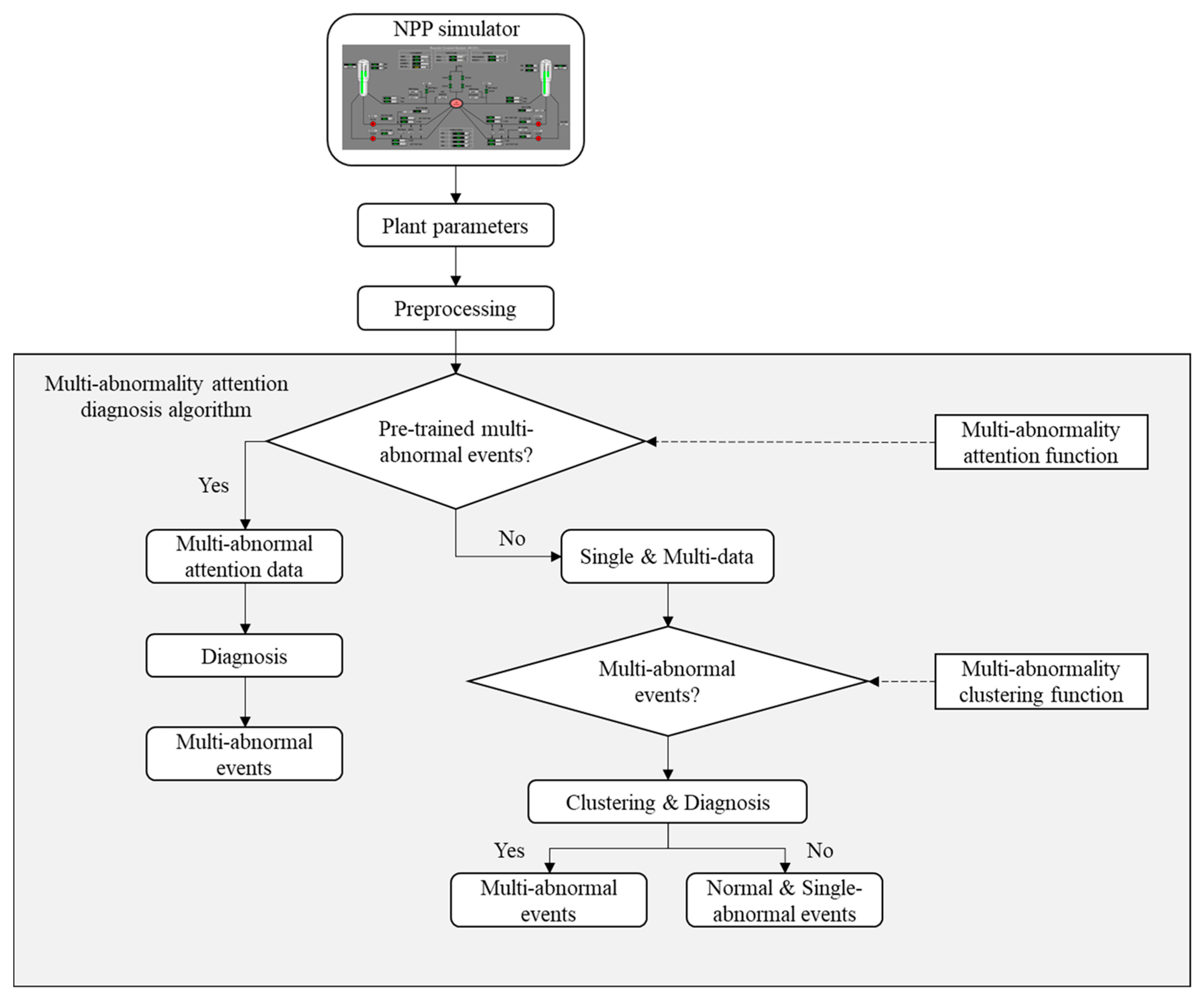
In this section, the hierarchical structure of the proposed multi-abnormality attention diagnosis model for effective and efficient operation is described in several stages. The term single-data is used to refer to normal and single abnormal data, while multi-abnormal data (or multi-data) reflects two different single abnormal data from two events occurring simultaneously during power operation. Figure 1 shows the overall framework of the multi-abnormality attention diagnosis model. The points below briefly introduce the framework.

• Data preprocessing: Raw data are preprocessed by feature extraction, normalization, and shape transformation. First, out of the plant parameters, feature extraction selects certain plant parameters to diagnose plant states. Then min–max normalization is applied due to large variations between plant parameters such as flow rate, temperature, electric power, and the number of pump rotations. Next, the procedure is adjusted to add the differences between the past and current plant parameter data into the OVR classifier, inspired by previous work [17]. See Section 3.2 for details.
• Multi-abnormality attention function: In this stage, we actively utilize the mean and standard deviation of the predicted probability distribution of the OVR model to deal with the multi-label classification problem. The OVR model trains only single-data first, and a predicted probability distribution is obtained from the validation dataset. The multi-abnormality attention function selects which multi-abnormal events should be trained additionally.
• Multi-abnormality clustering function: Test data are clustered into single- and multi-data by the multi-abnormality clustering function using the predicted probability distribution from the OVR model.
• Diagnosis: At the last stage of the proposed model, test data are diagnosed with the OVR model.

3.1. Multi-Label Classification via One-vs-Rest Classifier

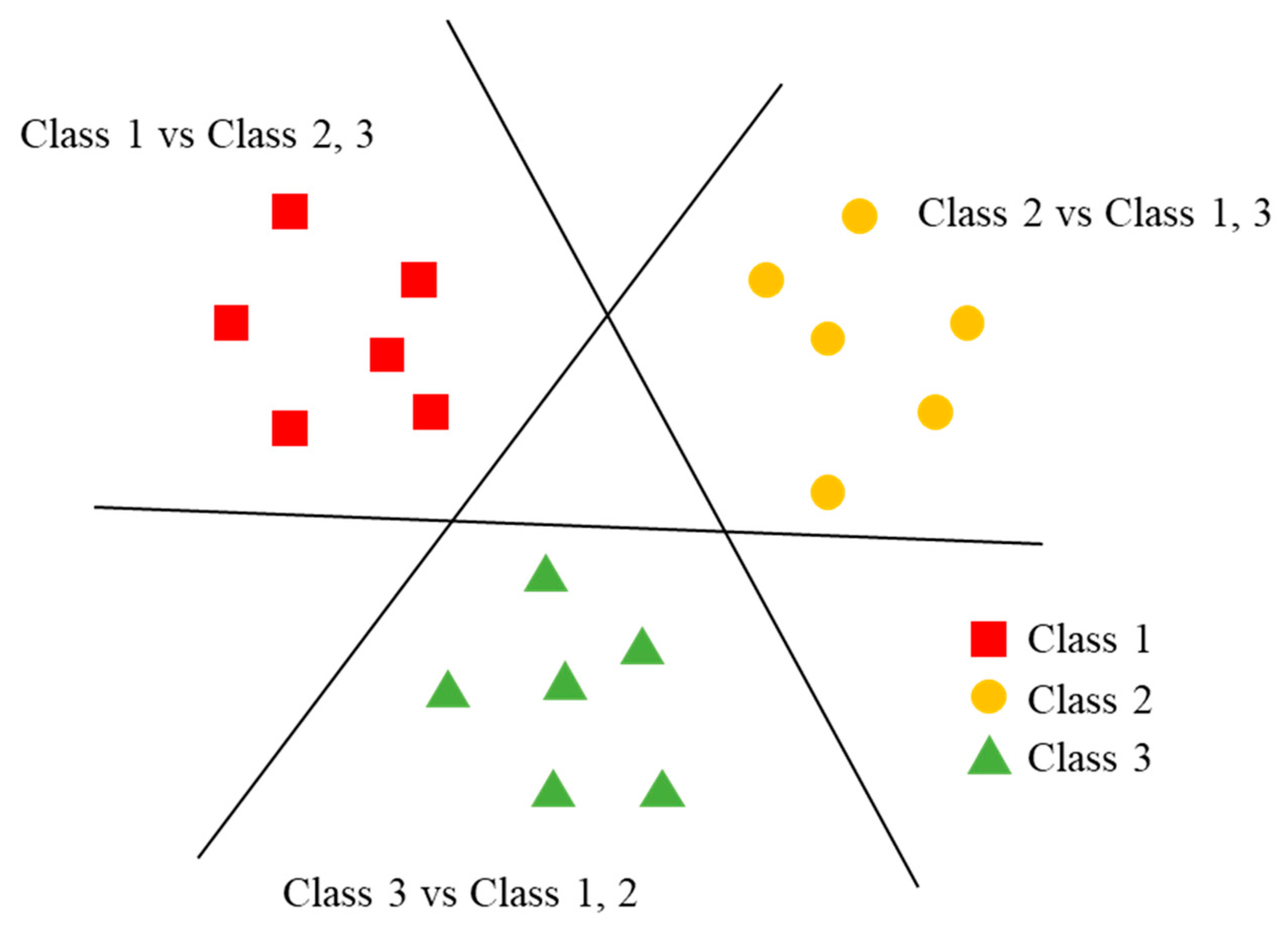
As shown in Figure 2, the OVR classifier requires as many SVM binary classifiers as there are class labels. The OVR classifier aims to set the decision boundary in the feature spaces between the labels; in Figure 2, the decision boundary is a hyperplane. The hyperplane is positioned as far as possible from the training labels.

Let ${\mathit{D}}_{\mathit{k}}=\left\{\left(x_1,y_{1k}\right),\left(x_2,y_{2k}\right), \dots , \left(x_n,y_{nk}\right)\right\}$ be the kth training dataset where $x_i$ is a feature vector and $y_{ik}$ is class label $i$ with $k=1, 2, \dots , m,$ $x_i\in {\mathit{R}}^d, \mathrm{and} y_i\in \left\{-1, 1\right\}$. The optimal hyperplane, which is handled as a decision boundary, can be obtained by Equation (1), where $w_k\in \mathit{W}=\left\{w_1,w_2, \dots , w_n\right\}$. $w_k$ is the weight vector and b_k is the bias.

$$f\left(x_i\right)=w_k{x}_i^T+b_k=0$$

(1)

The hyperplane should satisfy the following Equations (2) and (3) for arbitrary target label classes.

$$w_k{x}_i^T+b_k\ge 1, when y_{ik}=1$$

(2)

$$w_k{x}_i^T+b_k\ge -1, when y_{ik}=-1$$

(3)

These equations represent the margin of the hyperplane. To deal with overfitting problems of the hyperplane, the slack variables ${\xi }_{ik}\ge 0$ are introduced in Equation (4).

$$y_i\left(w_k{x}_i^T+b_k\right)-1+{\xi }_{ik}\ge 0$$

(4)

The objective function for maximizing the margin of the hyperplane can be represented as the following Equation (5), where C is a penalty variable to balance the classification accuracy and the complexity of the quadratic complexity of the hyperplane set.

$$\min \frac{{\left|\left|W_k\right|\right|}^2}{2}+C{{\displaystyle \sum }}_{i=1}^n{\xi }_{ik}, s.t. y_i\left(w_k{x}_i^T+b_k\right)-1+{\xi }_{ik}\ge 0$$

(5)

To solve Equation (5), Lagrange multipliers ${\lambda }_{ik}\ge 0$ are used, which can be expressed as the dual formula in Equation (6).

$$\max -\frac{1}{2}{{\displaystyle \sum }}_{i,j=1}^n{\lambda }_{ik}{\lambda }_{jk}{y}_{ik}{y}_{jk}\left(x_i^T{x}_j\right)+{{\displaystyle \sum }}_{i=1}^n{\lambda }_{ik}, s.t. {{\displaystyle \sum }}_{i=1}^n{\lambda }_{ik}{y}_{ik}=0, 0\le {\lambda }_{ik}\le C$$

(6)

Lastly, the decision function is defined as Equation (7).

$$label of x=\left\{k,s.t.w_k x_i^T+b_k\ge 0,k=1,2,\dots ,m\right\}$$

(7)

In our study, the OVR classifier is constructed using LibSVM tools for support vector regression [27,28].

3.2. Data Preprocessing

3.2.1. Data Normalization

Data preprocessing consists of data extraction, normalization, and transformation. Data extraction focuses on selecting plant parameters in consideration of NPP understanding and the degree of change in the parameters. The raw data produced by the simulator includes plant parameters according to each second. Parameters that typically do not change during abnormal events, such as safety injection tank level, aux feedwater pump mass flow rate, and others, may affect diagnostic accuracy and lead to unnecessary computational costs. Therefore, the relevant plant parameters that can be identified in the MCR are extracted first, and then all parameters in the normal and abnormal data that do not change are removed.

The types of plant parameters and ranges of parameter values are various, as mentioned earlier, so all plant parameters are normalized by the min–max scaling method using the minimum and maximum values of the nth plant parameter regardless of time in Equation (8). In this equation, ${\widehat{x}}_{t,n}$ is the value after normalization, where t is time and n is the nth plant parameter. Through the normalization process, the plant parameters have the same effect as a calculated weight vector.

$${\widehat{x}}_{t,n}=\frac{x_{t,n}-x_{\min of nth parameter }}{x_{\max of nth parameter }{}_{ }-x_{\min of nth parameter }}$$

(8)

3.2.2. Data Transformation (Two-Channel Model)

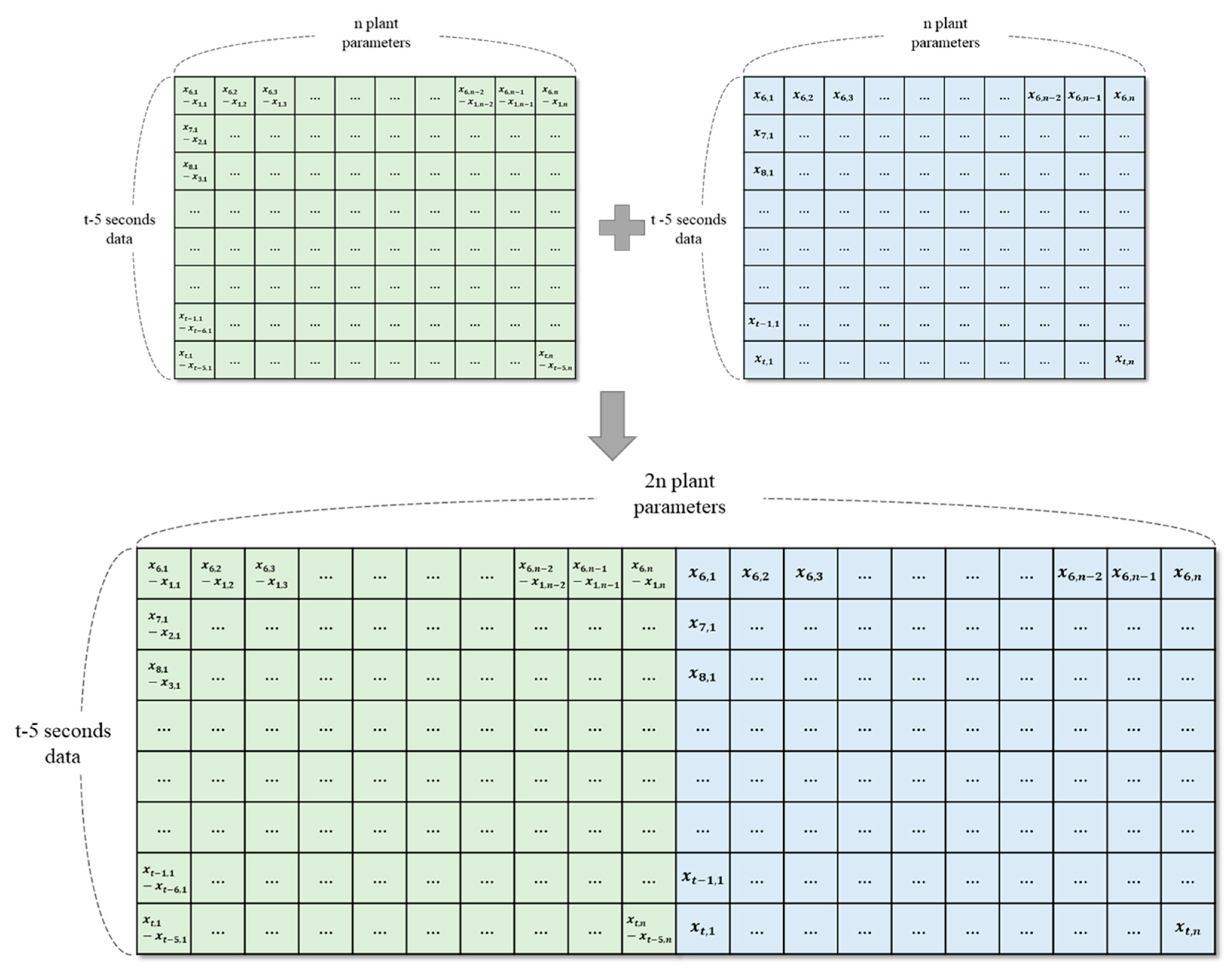
In reference [17], an abnormality diagnosis model was proposed using a two-channel CNN focused on transforming the data shape from the perspective of changes between past and present data to express the degree of variation of each parameter. Inspired by this work, we add the value of change from the past 5 s to the current value. Then the dataset $X_t=\left\{x_{t,1},x_{t,2},\dots ,x_{t,n}\right\}$ is the dataset at time t with n plant parameters. The transformed dataset can be represented in the following Equation (9) and Figure 3.

$$X_{t of transformed} =\left\{{\widehat{x}}_{t,1},{\widehat{x}}_{t,2},\dots ,{\widehat{x}}_{t,n}, \left({\widehat{x}}_{t,1}-{\widehat{x}}_{t-5,1}\right),\left({\widehat{x}}_{t,2}-{\widehat{x}}_{t-5,2}\right),\dots , \left({\widehat{x}}_{t,n}-{\widehat{x}}_{t-5,n}\right)\right\}$$

(9)

3.3. Multi-Abnormality Attention Diagnosis Algorithm

In this section, the detailed methodology for the multi-abnormality attention diagnosis algorithm of Figure 1 is described. This study aims to find which multi-labels are hard to classify and should be trained for high accuracy in an efficient manner; from now on, single-label refers here to a label for multi-class classification, and multi-label stands for a combined label of two different class labels. When the OVR classifier predicts the true label, the sum of the predicted probabilities becomes 1, and the probability distribution shows different aspects between single- and multi-labels. For instance, a well-fitted OVR classifier shows the highest predicted probability of close to 1 in the case of a single-label, but the highest predicted probability of a multi-label is lower than the single-label case. Focusing on this point, we use the distribution of the predicted probabilities of the OVR classifier to determine whether the data are single-label or multi-label and which multi-labels should be trained to get higher accuracy. The following paragraphs explain the overall multi-abnormality attention diagnosis algorithm including the multi-abnormality attention function and the multi-abnormality clustering function based on the OVR classifier.

The multi-abnormality attention function selects labels to convert the multi-label classification problem to a multi-class classification problem with additional training. Using the single-data validation set, we obtain the mean and standard deviation of the predicted probability for every single-label. Weights are given for a high mean predicted probability and penalties are given for a low standard deviation of the predicted probabilities because when the label does not fit well, the difference in predicted probabilities between single- and multi-labels is not large. Therefore, the multi-abnormal attention function is defined as Equation (10), where $n, l$ stand for the number of single-labels and the regulator constant, respectively. In the equation, $p_{L_i}$ is the predicted probability of multi-class label $L_i\left(i=1, 2, \dots n\right)$, and $p_{L_i,val, mean}$ and $p_{L_i,val, std}$ are the mean and standard deviation of the predicted probability of the validation dataset for the target label $L_i$, respectively.

$$if \left(1-p_{L_i,val, mean}\right)\times p_{L_i,val, std}>l\times \frac{1}{n}{{\displaystyle \sum }}_{j=1}^n\left(1-p_{L_j,val, mean}\right)\times p_{L_j, val,std}$$

(10)

The multi-labels are trained for multi-class classification if they contain a single-label that has the true value of the multi-abnormality attention function. Multi-labels with a false value from the multi-abnormality attention function proceed with multi-label classification using the multi-abnormality clustering function.

Clustering of single- and multi-labels is performed via the predicted probability distribution for each single-label corresponding to the multi-abnormality clustering function, Equation (11), using the mean and standard deviation of the predicted probability of the validation dataset for target label $L_i$.

$$\begin{gathered} Tested data is single label, if p_{L_i, test}>p_{L_i,val, mean}-k\times p_{L_i,val, std} \\ Tested data is multi label, if p_{L_i, test}\le p_{L_i,val, mean}-k\times p_{L_i,val, std} \end{gathered}$$

(11)

Here, $k$ is the regulator constant that determines how sensitive the model is to the multi-labels in terms of trade-offs with the single-labels. If the tested data is clustered as single-label, the OVR classifier performs multi-class classification; if the tested data are clustered as multi-label, the OVR classifier performs multi-label classification by diagnosing the top two predicted probability labels.

4. Experimental Settings

4.1. Description of Datasets

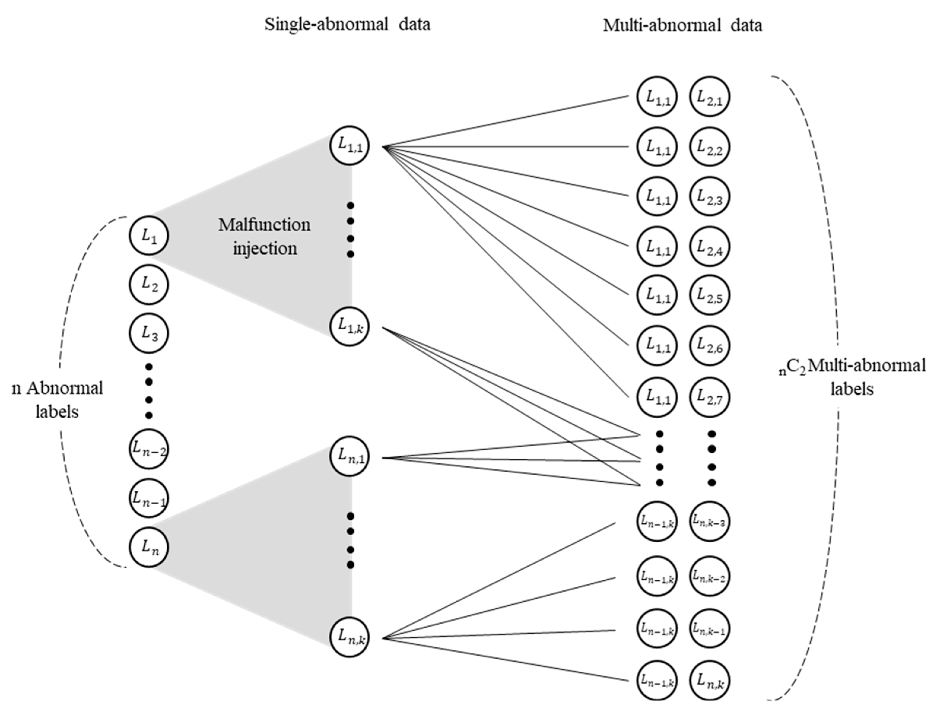
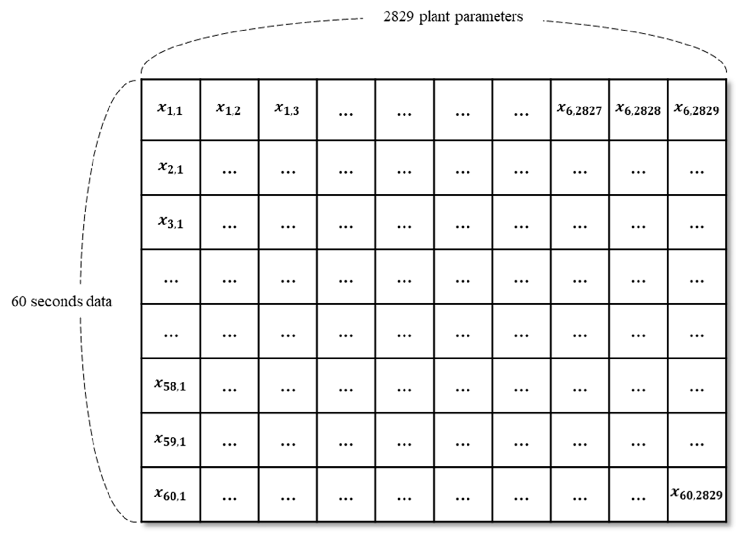
This study uses a PWR simulator to produce data instead of actual NPP operational data [29]. The 3KEYMASTER simulator made by Western Services Corporation models a generic two-loop 1400 MWe PWR. It can sufficiently simulate operation modes 1 to 5 and produce abnormal data through various malfunctions and device failures. The simulator is designed to allow users to drive desired scenarios through scenario codes. We use scenario codes to vary the degree of abnormality injection and the timing at which the injection is completed to produce normal, single-abnormal, and multi-abnormal data. The distinct cues of each abnormal data are inspected within 2 min, and we conservatively targeted 60 s of data for the experiment. Raw data from the simulator is generated in a matter of seconds and includes 2829 parameters indicating the state of the plant, such as mass flow rate, temperature, pressure, and others. Let $\mathit{L}=\left\{L_1,L_2,\dots ,L_n\right\}$ be the set of labels with the magnitude of malfunction $L_{i,j}\in \left\{L_{i,1},L_{i,2},\dots ,L_{i,7}\right\}$. Here, $i$, and $j$ represent the label and magnitude of the malfunction. Figure 4 shows the overall structure of the data produced using the simulator. Let ${\mathit{D}}_{\mathit{i},\mathit{j}}=\{x_{1,1},x_{1,2},\dots ,x_{60,2828},x_{60,2829}\}$ be the dataset with the label and magnitude of malfunction $i, j$ respectively. Then for an arbitrary label, $L_{i,j}$ has 2829 plant parameters within 60 s, as shown in Figure 5.

We produced single- and multi-abnormal events during the power operation of an NPP. Data production proceeded for a generic two-loop 1400 MWe PWR using the 3KEYMASTER simulator. We selected the abnormalities of the representative system-level abnormalities, and

Table 1. Data description.

Location of Abnormality Injection	Description	Main Symptoms
None (Normal)	Middle of the life cycle at 100% power generation	None
Steam generator tube leakage (SGTL)	Steam generator A tube leak	Secondary system radiation high, SG level high
Charging water system (CHRG)	Charging line break upstream	Charging line flowrate low, cavity sump level high
Letdown water system (LTDN)	Letdown line leak inside the containment	Letdown line flowrate low, cavity sump level high
Condensate system (CDS)	Loss of condenser vacuum	CDS pressure high, CDS hotwell temperature high
Pilot-operated safety relief valve (POSRV)	POSRV leak	PZR pressure low, POSRV discharging temperature high
Circulating water system (CWS)	Circulating water tube leak in low pressure condenser	CDS pressure high, CDS pit level high
Main steam isolation valve (MSIV)	MSIV positioner failure	SG pressure high, SG steam flowrate low
Reactor coolant pump (RCP)	RCP component cooling water service loop header leak to aux atm	CCW flowrate through RCP low
Main steam system (MSS)	Steam generator A steam line 1A break inside the containment	SG pressure low, SG steam flowrate low
Pressurizer (PZR)	PZR spray valve positioner failure	PZR pressure low, PZR spray temperature high
Component cooling water (CCW)	CCW service loop header leak to aux atm	CCW pump header discharging pressure low, CCW surge tank level low
Low-pressure feedwater heater (LFH)	Low feedwater heater 4A tube break	Low-pressure feedwater heater level high, condenser pump discharging pressure low
High-pressure feedwater heater (HFH)	High Feedwater heater 5A tube break	High-pressure feedwater heater level high, feedwater pump discharging pressure low
Main feed water (MFW)	MFW pump recirculating valve positioner open failure	SG level low, main feedwater pump drain flowrate high
Turbine control system (TCS)	High-pressure turbine control valve positioner close failure	Turbine power low, Tavg—Tref high

describes the abnormal events produced.

For each label, we produced 49 datasets consisting of about 2800 plant parameters over 60 s. Therefore, single-data has 1 normal and 15 single-abnormal events, giving a total of $16\times 49=784$ datasets. The data of the multi-abnormal events have a total of ${}_{15}{}^{}C{}_2\times 49=5148$ datasets through the combination formula of the single-abnormal events. Through the data extraction process, 467 plant parameters out of the approximately 2800 plant parameters were selected for the multi-abnormality attention diagnosis model. In addition, datasets for the two-channel model were converted into 467 × 2 plant parameters over 55 s instead of 60 s and 467 plant parameters in each dataset. For the training, validation, and test datasets, 70%, 10%, and 20% of the total data were used via random sampling, and all abnormal event datasets were used equally.

4.2. Description of Experimental Models

For a comparison of the proposed model, a CNN, FNN, and a one-vs-one (OVO) classifier, which is a type of SVM for multi-class classification, were included as a comparison group. Details of the architectures of these models are provided in the following

Table 2. Architecture of the OVR and OVO classifiers.

Characteristic	Description
Input size	(467, 1)
SVM type	Logistic regression
Solver	Liblinear

,

Table 3. Architecture of the CNN.

Characteristic	Description
Input size	(22, 22, 1)
Kernel size	(3, 3)
Max pooling size	(2, 2)
Number of conv 2D layers	2
Number of max pooling 2D layers	2
Number of dense layers	2
Loss function	Binary cross-entropy
Activation function	ReLU, sigmoid
Optimizer	Adam
Epochs	100
Early stopping	30
Learning rate	0.001

and

Table 4. Architecture of the FNN.

Characteristic	Description
Input size	(467, 1)
Number of layers	2
Number of max pooling layers	2
Number of dense layers	2
Loss function	Binary cross-entropy
Activation function	ReLU, sigmoid
Optimizer	Adam
Epochs	100
Early stopping	30
Learning rate	0.001

.

4.3. Evaluation Method via Confusion Matrix

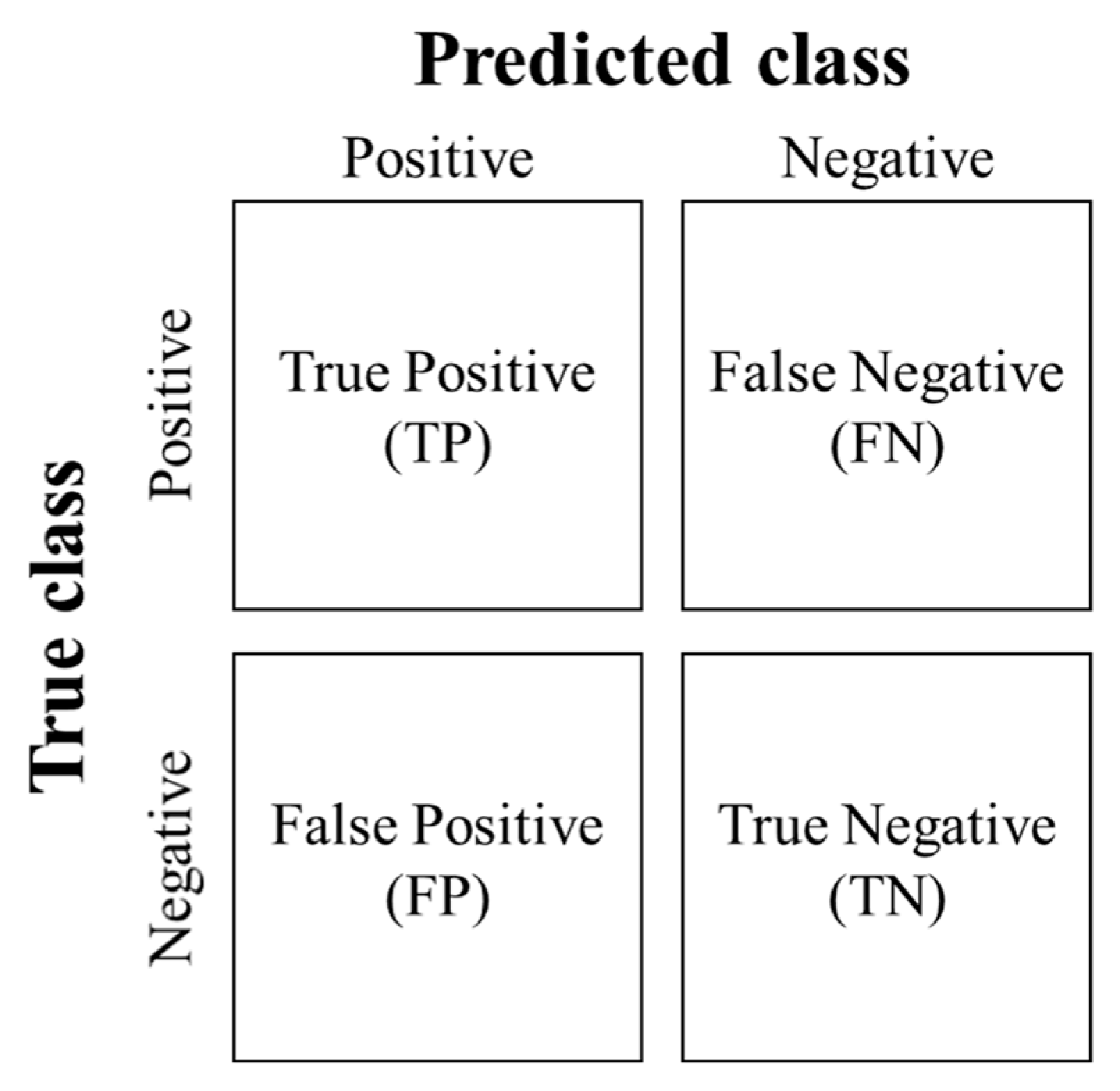
Evaluation of each model was carried out using a confusion matrix. However, instead of obtaining a confusion matrix for each label, we obtained a confusion matrix for the models. The following metrics and Equations (12)–(15) show the evaluation methods of accuracy, precision, recall, and F1 score for the models according to Figure 6, showing label L_i (i = 1, 2,…, n) for a number of labels n.

• Accuracy: ratio of correctly classified classes to all classes

  $$\mathrm{Accuracy}=\frac{1}{n}{{\displaystyle \sum }}_{i=1}^n\frac{T{P}_{L_i}+T{N}_{L_i}}{T{P}_{L_i}+T{N}_{L_i}+F{P}_{L_i}+F{N}_{L_i}}$$
• Precision: ratio of correctly predicted classes to predicted positive classes

  $$\mathrm{Precision}=\frac{1}{n}{{\displaystyle \sum }}_{i=1}^n\frac{T{P}_{L_i}}{T{P}_{L_i}+F{P}_{L_i}}$$
• Recall: ratio of correctly classified classes to true positive classes

  $$\mathrm{Recall}=\frac{1}{n}{{\displaystyle \sum }}_{i=1}^n\frac{T{P}_{L_i}}{T{P}_{L_i}+F{N}_{L_i}}$$
• F1 score: harmonic mean of precision and recall

  $$\mathrm{F}1 \mathrm{score}=\frac{1}{n}{{\displaystyle \sum }}_{i=1}^n\frac{2\times precisio{n}_{L_i}\times recal{l}_{L_i}}{precisio{n}_{L_i}+recal{l}_{L_i}}$$

5. Results

In this section, the performance of each AI model for the multi-class classification of normal and single abnormal events is first verified. Based on the results, we select the AI models to be used for multi-abnormal events and validate their performance in multi-label classification. We then train additional multi-abnormal data via the proposed multi-abnormality attention function for selective training and test the multi-abnormality attention diagnosis model, showing the amount of data used and its accuracy.

5.1. Model Performance Comparison for Single-Abnormality Diagnosis

The presented models for single-abnormality diagnosis are of two types, namely one-channel and two-channel. The two-channel models are to additionally reflect the difference between the current plant parameters and those from 5 s before. Therefore, the one-channel models perform diagnosis for 600 s for each normal and abnormal state, which is 20% of the total data, and the two-channel models perform diagnosis for 550 s for each normal and abnormal state, which is 20% of the total data. In the case of the CNN and FNN models, binary cross-entropy loss and sigmoid activation functions were used to advance to multi-label classification.

Table 5. Results of the single-abnormality diagnosis models with one channel.

Model	OVR	OVO	CNN	FNN
Accuracy	0.9804	0.9756	0.9824	0.9705
Precision	0.9806	0.97625	0.9838	0.9719
Recall	0.98	0.9756	0.9825	0.97
F1 score	0.98	0.975	0.9819	0.9694

and

Table 6. Results of the single-abnormality diagnosis models with two channels.

Model	2ch-OVR	2ch-OVO	2ch-CNN	2ch-FNN
Accuracy	0.9978	0.9976	1	0.9931
Precision	0.9975	0.9975	1	0.9938
Recall	0.9975	0.9975	1	0.9931
F1 score	0.9975	0.9975	1	0.9938

list the results of the one- and two-channel models, respectively, trained with normal data and 15 single-abnormal data. In this study, the one-channel models adopt data that have been preprocessed via Equation (8), and the two-channel models adopt data that has been preprocessed via Equation (9), as described in Figure 3. In the case of the CNN, the input shape was (22,22,2), while the input shapes of the other models were (467 × 2).

Before implementation of the multi-abnormality diagnosis model, the initial single-abnormality diagnosis experiment was conducted to confirm the baseline performance of the models. The results show that the two-channel models reflecting the difference between current and past data have better performance than the one-channel models, and also that the OVR classifier among the SVM models and the CNN among the neural network models have excellent performance. Therefore, the OVR and CNN were selected for implementation in the multi-abnormality diagnosis model; their results are compared in the next section.

Table 7. Results of the single-abnormality diagnosis model with two-channel OVR classifier.

Location of Abnormality Injection	Accuracy	Precision	Recall	F1 Score
None (normal)	1	0.96	1	0.98
Steam generator tube leakage (SGTL)	1	1	1	1
Charging water system (CHRG)	1	1	1	1
Letdown water system (LTDN)	1	1	1	1
Condensate system (CDS)	1	1	1	1
Pilot-operated safety relief valve (POSRV)	1	1	1	1
Circulating water system (CWS)	1	1	1	1
Main steam isolation valve (MSIV)	1	1	1	1
Reactor coolant pump (RCP)	0.964	1	0.96	0.98
Main steam system (MSS)	1	1	1	1
Pressurizer (PZR)	1	1	1	1
Component cooling water (CCW)	1	1	1	1

shows the label-specific performance of the two-channel OVR model for single-abnormality diagnosis.

5.2. Multi-Abnormality Attention Diagnosis Model

The results of the previous section showed that the best model for multi-class classification was the two-channel CNN, but in the case of multi-abnormality diagnosis, this model can come with a disadvantage due to overfitting problems for single abnormal events. For the sigmoid activation function, the predicted probability for all labels is expressed between 0 and 1, so single and multi-abnormal events are divided according to the abnormal events with predicted probabilities higher than a certain threshold. For instance, if the second-highest predicted probability is greater than the threshold value, the test data are classified as a multi-abnormal event, and the two highest abnormal events are diagnosed. However, even with different threshold values set, the two-channel CNN was weak at multi-abnormality diagnosis problems, as the results in

Table 8. Accuracy of the multi-abnormality diagnosis models with two-channel CNN.

Accuracy	Two-Channel CNN with Threshold 0.5	Two-Channel CNN with Threshold 0.1
Single-data	1	1
Multi-data	0.138	0.168
Total data	0.2524	0.2783

show. Therefore, the OVR model was adopted as the model for clustering and diagnosing multi-abnormal data.

The method for clustering single and multi-abnormal events was introduced in Section 3.3 using the multi-abnormality clustering function that includes the regulator constant k from Equation (11). To select the regulator constant k, values were tested from 1 to 5 at intervals of 0.5, and values with an accuracy higher than 95 percent for single-data were chosen. The obtained values were 2.5 and 3, with which the diagnosis results of single-data after clustering are compared between the CNN and OVR models. The CNN model is used at the multi-class classification level after clustering the single- and multi-abnormal labels. Corresponding to the value of k, the accuracy of the single- and multi-abnormal data varies in terms of trade-offs. Since the accuracy is higher when the OVR model is used alone, as shown in

Table 9. Accuracy of the multi-abnormality diagnosis models.

Accuracy	CNN + OVR with k = 2.5	CNN + OVR with k = 3	OVR with k = 2.5	OVR with k = 3
Single-data	0.96	0.971	0.97	0.977
Multi-data	0.855	0.834	0.859	0.838
Total data	0.855	0.852	0.873	0.856

, the OVR model is used alone in the subsequent experiments.

The multi-abnormality attention function selects the multi-abnormal events to be trained for multi-class classification, and the regulator constant $l$ is set to 1. Figure 7 shows the multi-abnormality attention scores of each abnormal event, where the multi-abnormality attention events contain SGTL, RCP, and PZR (see Table 1). The accuracies of SGTL, RCP, and PZR, which have true values of the multi-abnormality attention function, were the worst because of the large standard deviation and the small mean value of their predicted probabilities during the clustering phase of the single- and multi-abnormal events of Equation (11).

Table 10. Accuracy of the multi-abnormality attention diagnosis models.

Accuracy	OVR Model with k = 2.5, l = 1	OVR Model with k = 3, l = 1
Single-data	0.97	0.977
Multi-data	0.981	0.98
Total data	0.979	0.98

presents the accuracy of the proposed multi-abnormality attention diagnosis model, showing the highest accuracy for $k$ = 3, $l$ = 1.

Now, the proposed multi-abnormality attention diagnosis model is compared with the other two types of multi-abnormality diagnosis models, namely those trained on only single-data and those trained on all single- and multi-data, in terms of data usage and diagnostic accuracy. Because training all single- and multi-data diagnosis models belongs to multi-class classification, the best-performing two-channel CNN model for a single abnormal event was used.

Table 11. Comparison of multi-abnormality diagnosis models.

Result	OVR Model with $\mathit{k}$ = 3	OVR Model with $\mathit{k}$ = 3, $\mathit{l}$ = 1	CNN Model with All Data Trained
Accuracy of single-data	0.970	0.977	0.938
Accuracy of multi-data	0.859	0.980	1.000
Accuracy of total data	0.873	0.980	0.992
% of data usage to all data Time (s)	13.22% (29,920 s)	45.45% (102,850 s)	100% (226,270 s)

shows the comprehensive results of the multi-abnormality diagnosis models. AI models perform better depending on the quantity and quality of the training data, so the CNN trained on all single- and multi-data for multi-class classification shows the highest accuracy due to a large amount of training data. However, training all kinds of multi-abnormal data is an inefficient and impractical way to increase the diagnostic accuracy of the model for multi-abnormal events. For instance, as mentioned earlier, the APR-1400 has 82 AOPs with 224 sub-procedures, giving a total of ${}_{224}{}^{}C{}_2=24,976$ possible multi-abnormal events by the combination formula. Such a huge number for multi-class classification can decrease the performance of the diagnosis model. 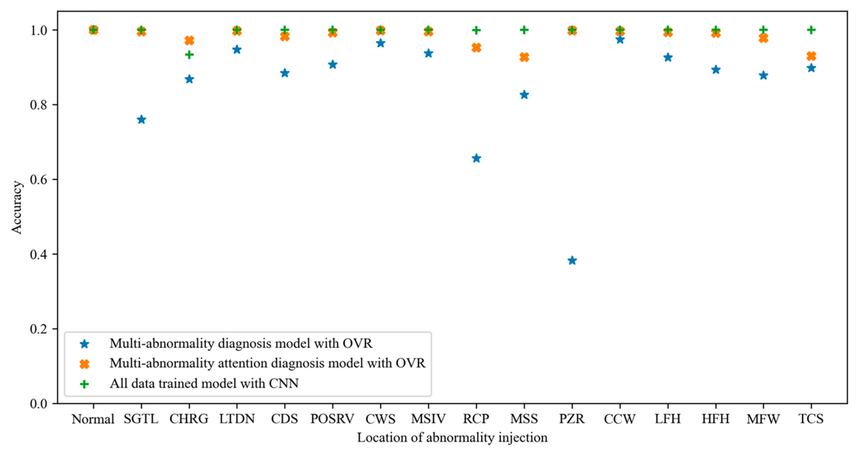Figure 8 shows the accuracy of the diagnosis models for each label, including single- and multi-abnormal data. When performing diagnosis using the predicted probability distribution with only single-data, the amount of data used is as low as 13.22% of the total data, but this shows relatively low accuracy. Conversely, the diagnosis model using all data is highly accurate but inefficient in producing and training data. Moreover, for diagnosis models that have trained too many labels, the accuracy for a single abnormal event decreases in the all-data-trained CNN model of Table 11. The proposed multi-abnormality attention diagnosis model trained only 45.45% of the total data but, similar to the CNN trained on all data, shows an accuracy of 98%.

6. Conclusions

In the power operation mode of NPPs, operators should select the appropriate AOP when an abnormal event occurs. However, in the case of the APR-1400, 224 sub-procedures of 82 AOPs and thousands of plant parameters can lead to operator stress and possible event misdiagnosis. Accordingly, operator support systems using AI in various ways are being studied to reduce human error, but multi-abnormality diagnosis problems have not been mentioned due to their rare incidence. The occurrence of multi-abnormal events does not correspond to the entry conditions of general AOPs, which are fitted to a typical single abnormal event, and the consequent nonlinear NPP parameters would pose a heavy burden on operators.

To deal with these problems, this study proposed an efficient way to diagnose multi-abnormal events using predicted probability distributions from an OVR classifier. The diagnosis of multi-abnormal events is a type of multi-label classification problem, for which diagnosis is very difficult by training only single abnormal events. Therefore, we also presented a method for selectively training multi-abnormal events because of the inefficiency of training all multi-abnormal events. Before the diagnosis of multi-abnormal events, single-abnormality diagnosis models based on OVO, OVR, FNN, and CNN architectures were first compared. Accuracy was improved through the consideration of additional parameters, including changes between past and present plant parameters. Among the single-abnormality diagnosis models, the OVR (a type of SVM) and CNN (a type of neural network) were selected as candidates for the multi-abnormality diagnosis model. The results of the multi-abnormality diagnosis model using the predicted probability distributions of the OVR model were the best, showing about 87% accuracy. Furthermore, the presented multi-abnormality attention function was able to recognize which multi-abnormal events are difficult to diagnose or unpredictable and require additional training. The multi-abnormality attention diagnosis model achieved 98% accuracy by training only about 45% of the total data, which is very close to the 99.2% accuracy of the model trained on all the data. The proposed methods can provide insight to NPP operators to better cope with multi-abnormal events and, in this way, can contribute to improving nuclear safety as an operator support system with a decision-making tool.

Despite the remarkable identification performance of the multi-abnormality attention diagnosis model, diagnosing multiple abnormalities in NPPs is still a challenging problem, considering the highly complex and dynamic trends. To apply the proposed model to actual plants as an operator support system, the following items should be further studied. (1) In this work, we preferentially selected and tested representative system-level abnormalities. In the future, more abnormal events will need to be diagnosed in consideration of high accuracy. (2) Methods to efficiently use computer resources are needed to track changing variables and diagnose various abnormalities, such as optimizing the number of hyper-parameters or separately training the multi-abnormalities with high priority. (3) Unlike real plants, simulators consist of noise-free data and can produce as much data as desired. For AI models trained with simulator data only, applying the models to real-world plants requires additional efforts to manage noise or develop robust models. If possible, it would be best to train actual plant data. (4) Following the multi-abnormality diagnosis, a systematic execution list for each abnormality is necessary to facilitate the rapid escape from the multi-abnormal events and restore safe plant operation.

References

- Lee, S.-J.; Seong, P.-H. Development of an integrated decision support system to aid cognitive activities of operators. Nucl. Eng. Technol. 2007, 39, 703–716. [Google Scholar] [CrossRef]
- Le Bot, P. Human reliability data, human error and accident models—Illustration through the Three Mile Island accident analysis. Reliab. Eng. Syst. Saf. 2004, 83, 153–167. [Google Scholar] [CrossRef]
- Xu, H.; Zhang, B. A review of the FLEX strategy for nuclear safety. Nucl. Eng. Des. 2021, 382, 111396. [Google Scholar] [CrossRef]
- Shin, J.H.; Kim, J.M.; Lee, S.J. Abnormal state diagnosis model tolerant to noise in plant data. Nucl. Eng. Technol. 2021, 53, 1181–1188. [Google Scholar] [CrossRef]
- Kim, J.M.; Lee, G.; Lee, C.; Lee, S.J. Abnormality diagnosis model for nuclear power plants using two-stage gated recurrent units. Nucl. Eng. Technol. 2020, 52, 2009–2016. [Google Scholar] [CrossRef]
- Zhang, M.L.; Li, Y.K.; Liu, X.Y.; Geng, X. Binary relevance for multi-label learning: An overview. Front. Comput. Sci. 2018, 12, 191–202. [Google Scholar] [CrossRef]
- Hsieh, M.H.; Hwang, S.L.; Liu, K.H.; Liang, S.F.M.; Chuang, C.F. A decision support system for identifying abnormal operating procedures in a nuclear power plant. Nucl. Eng. Des. 2012, 249, 413–418. [Google Scholar] [CrossRef]
- Kang, J.S.; Lee, S.J. Concept of an intelligent operator support system for initial emergency responses in nuclear power plants. Nucl. Eng. Technol. 2022, 54, 2453–2466. [Google Scholar] [CrossRef]
- Moro, S.; Cortez, P.; Rita, P. A data-driven approach to predict the success of bank telemarketing. Decis. Support Syst. 2014, 62, 22–31. [Google Scholar] [CrossRef]
- Bae, J.; Kim, G.; Lee, S.J. Real-time prediction of nuclear power plant parameter trends following operator actions. Expert Syst. Appl. 2021, 186, 115848. [Google Scholar] [CrossRef]
- Abiodun, O.I.; Jantan, A.; Omolara, A.E.; Dada, K.V.; Umar, A.M.; Linus, O.U.; Arshad, H.; Kazaure, A.A.; Gana, U.; Kiru, M.U. Comprehensive review of artificial neural network applications to pattern recognition. IEEE Access 2019, 7, 158820–158846. [Google Scholar] [CrossRef]
- El-Sefy, M.; Yosri, A.; El-Dakhakhni, W.; Nagasaki, S.; Wiebe, L. Artificial neural network for predicting nuclear power plant dynamic behaviors. Nucl. Eng. Technol. 2021, 53, 3275–3285. [Google Scholar] [CrossRef]
- Ho, L.V.; Nguyen, D.H.; Mousavi, M.; De Roeck, G.; Bui-Tien, T.; Gandomi, A.H.; Wahab, M.A. A hybrid computational intelligence approach for structural damage detection using marine predator algorithm and feedforward neural networks. Comput. Struct. 2021, 252, 106568. [Google Scholar] [CrossRef]
- Zhang, J.; Xie, Y.; Wu, Q.; Xia, Y. Medical image classification using synergic deep learning. Med. Image Anal. 2019, 54, 10–19. [Google Scholar] [CrossRef]
- Altwaijry, N.; Al-Turaiki, I. Arabic handwriting recognition system using convolutional neural network. Neural Comput. Appl. 2021, 33, 2249–2261. [Google Scholar] [CrossRef]
- Wu, J. Introduction to convolutional neural networks. Natl. Key Lab Nov. Softw. Technol. Nanjing Univ. China 2017, 5, 495. [Google Scholar]
- Lee, G.; Lee, S.J.; Lee, C. A convolutional neural network model for abnormality diagnosis in a nuclear power plant. Appl. Soft Comput. 2021, 99, 106874. [Google Scholar] [CrossRef]
- Huang, S.; Cai, N.; Pacheco, P.P.; Narrandes, S.; Wang, Y.; Xu, W. Applications of support vector machine (SVM) learning in cancer genomics. Cancer Genom. Proteom. 2018, 15, 41–51. [Google Scholar]
- Ahmad, A.S.; Hassan, M.Y.; Abdullah, M.P.; Rahman, H.A.; Hussin, F.; Abdullah, H.; Saidur, R. A review on applications of ANN and SVM for building electrical energy consumption forecasting. Renew. Sustain. Energy Rev. 2014, 33, 102–109. [Google Scholar] [CrossRef]
- Ameer, I.; Sidorov, G.; Gomez-Adorno, H.; Nawab, R.M.A. Multi-label emotion classification on code-mixed text: Data and methods. IEEE Access 2022, 10, 8779–8789. [Google Scholar] [CrossRef]
- Hussain, S.F.; Ashraf, M.M. A novel one-vs-rest consensus learning method for crash severity prediction. Expert Syst. Appl. 2023, 228, 120443. [Google Scholar] [CrossRef]
- Wang, Y.; Sun, P. A fault diagnosis methodology for nuclear power plants based on Kernel principle component analysis and quadratic support vector machine. Ann. Nucl. Energy 2023, 181, 109560. [Google Scholar] [CrossRef]
- Tax, D.M.; Duin, R.P. Support vector data description. Mach. Learn. 2004, 54, 45–66. [Google Scholar] [CrossRef]
- Wang, J.; Yang, Y.; Mao, J.; Huang, Z.; Huang, C.; Xu, W. Cnn-rnn: A unified framework for multi-label image classification. In Proceedings of the IEEE Conference on Computer Vision and Pattern Recognition, Las Vegas, NV, USA, 27–30 June 2016; pp. 2285–2294. [Google Scholar]
- Jang, J.; Kim, C.O. One-vs-rest network-based deep probability model for open set recognition. arXiv 2020, arXiv:2004.08067. [Google Scholar]
- Xu, J. An extended one-versus-rest support vector machine for multi-label classification. Neurocomputing 2011, 74, 3114–3124. [Google Scholar] [CrossRef]
- Abdiansah, A.; Wardoyo, R. Time complexity analysis of support vector machines (SVM) in LibSVM. Int. J. Comput. Appl. 2015, 128, 28–34. [Google Scholar] [CrossRef]
- Chang, C.-C.; Lin, C.-J. LIBSVM: A library for support vector machines. ACM Trans. Intell. Syst. Technol. (TIST) 2011, 2, 1–27. [Google Scholar] [CrossRef]
- Western Service Corporation. 3KEYMASTER Simulator; Western Service Corporation: Frederick, MD, USA, 2013. [Google Scholar]