Application of Machine Learning for Classification of Nuclear Reactor Operational Status Using Magnetic Field Sensors

Abstract

The nuclear fuel cycle forms the basis for producing special nuclear materials used in nuclear weapons via a series of interdependent industrial operations. These industrial operations each produce characteristic emanations that can be gathered to ascertain signatures of facility operations. Machine learning and deep learning techniques were applied to time series magnetic field sensor data collected at the High Flux Isotope Reactor (HFIR) to assess the feasibility of determining the ON/OFF operational state of the reactor. When data collected by the sensor near the cooling fans, position 9, are transformed to the frequency domain, it was found that both machine and deep learning methods were able to classify the operational state of the reactor with a balanced accuracy of over 90%. This result suggests that the utilized methods show promise for application as techniques to verify declared activities involving nuclear reactors. Additional effort is recommended to develop models and architectures that will more fully capitalize on the data’s temporal nature by incorporating the magnetic field’s time dependence to improve the model’s robustness and classification performance.

1. Introduction

In an age of scientific and engineering advancements, the United States of America is far from the only nation with nuclear capabilities [1]. Since the Manhattan project, the spread of basic nuclear science and technology has resulted in nuclear weapon proliferation as well as the spread of peaceful nuclear applications. Along with this spread, treaties and agreements to slow or stop testing and nuclear proliferation have also been agreed upon, such as the Treaty on the Non-Proliferation of Nuclear Weapons (NPT) and the Comprehensive Nuclear-Test-Ban Treaty (CTBT) [2,3]. The current method of assessing compliance with the NPT is through the International Atomic Energy Agency (IAEA) which safeguards nuclear materials and monitors activities in more than 140 countries [4]. As the first step in guarding against diversion of materials towards nuclear weapons development, treaty verification requires gathering data about an actor’s use of nuclear technologies to give insight into potential applications.

Advanced data analysis techniques can assist in verifying whether the information collected is consistent with stated declarations. Previous research conducted by the Multi-Informatics for Nuclear Operating Scenarios (MINOS) venture explored methods of monitoring activities at nuclear reactor sites to promote nuclear treaty monitoring objectives. As an example, activities at nuclear reactors have been monitored using physical signals such as infrasound and low-frequency acoustic signals. Cárdenas et al. investigated the use of smartphones and a cloud-based architecture to detect activities near nuclear reactors such as crane operations, opening and closing of access doors, and vehicle operations in the reactor vicinity utilizing sensor networks [5]. The research found that airlock door activity could be identified using a two-sample t-test in conjunction with timing analysis to trigger a notification algorithm using local acoustic sensors. Members of the same group performed a subsequent study that assessed the monitoring of a nuclear reactor during full power generation utilizing a similar network of sensors for infrasound and low-frequency acoustic signals [6]. A fundamental frequency of 21.4 Hz was found to be associated with dual-speed cooling fan operations indicative of the reactor power status and was observed up to ∼900 m from the cooling tower. Gastelum et al. performed similar studies with two data streams, open source image data and multi-modal sensing platforms for indirect physical sensing [7]. The study looked at both data streams individually and then as one integrated analysis to assess the potential benefit of multi-modal fusion approaches. Eaton et al. used locally collected infrasound measurements to predict the operation of mechanical draft cooling towers associated with nuclear reactors which are critical for managing heat in the reactor [8]. The approach was tested using data from the Advanced Test Reactor at Idaho National Laboratory and the High Flux Isotope Reactor at Oak Ridge National Laboratory. It was found that the developed algorithm could successfully be used to predict fan speed and active cooling capacity.

Machine Learning (ML) and Deep Learning (DL) are also being employed to characterize nuclear reactor operations. One example from Tibbets et al. exploits a data stream from the same multi-sensor network used in the present work collected in the vicinity of the High Flux Isotope Reactor (HFIR) at Oak Ridge National Laboratory [9]. The reactor’s operational state (ON/OFF) was classified using a DL feed-forward network trained on time series sensor data. A binary classification accuracy of $88.4\%$ was obtained. A corresponding feature importance study concluded that the magnetic field data was the most important contributing factor to the classification accuracy. Chai et al. used ML to predict a reactor’s operational state using seismic and acoustic data [10]. The study made use of ML models such as linear regression, k-nearest neighbors, gradient boosting, and random forests with features that had been selected in both the time-domain and frequency-domain. A binary, ON/OFF, classification accuracy of 98% was achieved with a gradient boosted algorithm with fusion of both seismic and acoustic data. Going beyond the binary problem, Rao et al. used a ML model to predict the power level of a reactor given features from a data fusion technique trained on data from infrared, electromagnetic, and acoustic sensors [11]. Their estimator achieved $3.47\%$ or lower root mean square error utilizing a 5-fold cross validation for determination of reactor power level.

Classification of nuclear reactor operational state is not the only use case for ML in a nuclear setting. Calivá et al. used DL to detect anomalies in nuclear reactors, such as changes in process parameters like neutron flux to gain insight into the functionality of the core [12]. This work used simulated neutron noise in a pressurized water reactor core fed into convolutional neural networks (CNNs) and clustering algorithms such as k-means to unfold the generated signals, followed by a denoising auto-encoder to reconstruct power reactor signals with various noise levels and corruption. This process resulted in an accuracy of 95.3% for twelve classes of perturbation location sources. Another example of ML studies with nuclear reactor data is from Zhong et al. [13]. The study used transfer learning of a convolutional neural network pre-trained on a database for fault diagnosis and accident identification, an area which has very little native data with which to work. The transfer learning technique was proposed to mitigate that problem.

The method of investigation proposed in this research is to employ ML and DL to classify whether a nuclear reactor is powered ON or OFF, based on data collected using passive persistent sensors. This study leverages the results presented by Tibbets et al. by focusing on the magnetic field data since it was found to be the most significant phenomenology contributing to the binary classification accuracy [9]. In contrast to the previous work, a frequency domain analysis is presented.

2. Materials and Methods

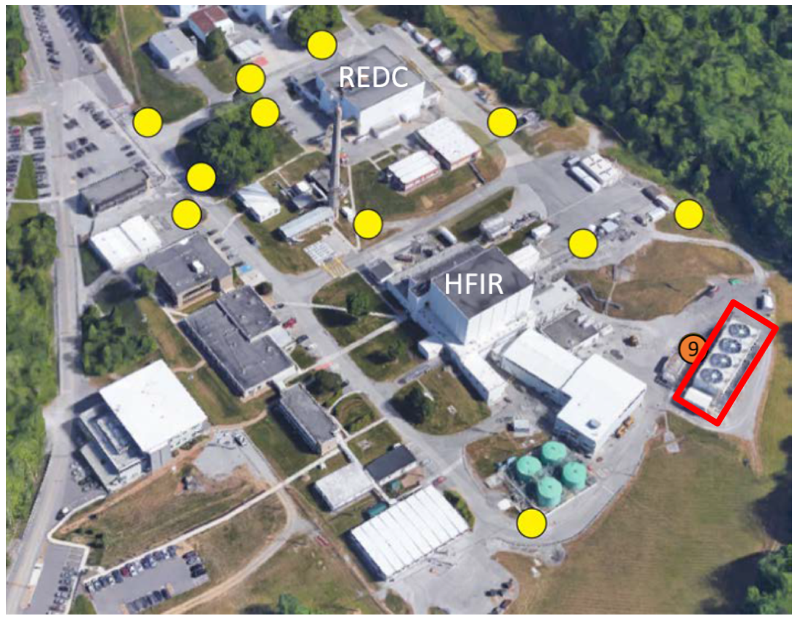
The reactor under examination is the High Flux Isotope Reactor (HFIR) at Oak Ridge National Laboratory. Twelve sensors have been placed in the area around the reactor as shown in Figure 1. They collect information about physical phenomena such as the magnetic field in three axes $B(x,y,z)$, seismic acceleration in three axes $a(x,y,z)$, pressure, temperature, ambient light, color (RGB + UV) and proximity [7].

The magnetometers at position 9 shown by the orange circle were selected for analysis due to their proximity to the cooling fans. The duty cycle and variable speed of the cooling fans is expected to reflect the operational load of the facility. When the cooling fans operate, they use electricity. The flow of electricity produces a magnetic field. The magnetic field data was collected via 3 magnetometers positioned to collect along the x, y, and z axes at this location. The positive z-axis pointed from the cooling fans towards the HFIR, the positive y-axis pointed along the cooling fans towards the right of the image, and the positive x-axis pointed toward the sky. The data coming from the sensors is in a time-series stream, recording measurements at a rate of 16 Hz. The experiment described next creates a function which maps the signals recorded by the sensor to the facility status. The fan status is unknown.

The time frame over which data for this work was selected comes from four operational cycles of the HFIR, shown in

Table 1. The operational cycles of the HFIR reactor considered in this paper. Each cycle spans 32+ days with data measured at a 16 Hz rate, which provided enough data for the ML and DL approaches.

HFIR Cycle	Start Date	End Date	nDays in Cycle	nDays between Cycles
484	29 Oct 2019	29 Nov 2019	32	N/A
485	28 Apr 2020	06 Jun 2020	39	181
486	23 Aug 2020	30 Sep 2020	38	78
488	03 Mar 2021	04 Apr 2021	32	154

. Cycles 484, 485, and 486 were used to create training and testing sets, with Cycle 488 kept isolated for further testing and model verification. During each cycle, the HFIR was gradually powered up until it reached full power. The reactor was run at full power for approximately 27 days, then gradually powered down reaching its OFF state. During the OFF period, data were collected for approximately 5 days with no other systems changing. In this study, the ON class refers to the period when the reactor power is >7%, and the OFF class refers to when the reactor power is ≤7%. The 7% threshold for ON and OFF classes was based off a process by the data owners and is an inherited number. The sensitivity of this research to the threshold will be explored in the future. A class imbalance was present within the data with a greater number of measurements taken in the ON state than the OFF state. This will be accounted for in the analysis.

Data Preprocessing

The first step in preprocessing the data for input into a ML or DL model was to convert the 3-axis magnetic field data into a magnetic field magnitude via Equation (1). That is to say that each 16th of a second, magnetic field components measured in the $B_x$, $B_y$, and $B_z$ directions were converted into magnitude using Equation (1). This step was done to decrease the dimensionality of the data, due to the total number of features resulting from the next preprocessing step.

$$\mathbf{B}\left(t\right)=\sqrt{B_x^2+B_y^2+B_z^2}$$

(1)

The frequency domain may contain features indicative of a reactor’s operational state. For instance, transforming the data into the frequency domain, one can look at how often a frequency occurs within any given measurement. To use this data in the frequency domain, a Short Time Fourier Transform (STFT) was applied. Similar to a moving window of calculations, the STFT takes a range of time sampled data and converts it into a frequency spectrum with granularity dependent on the length of samples given [14]. The amount of time series data given to the STFT must be at least one second, per the 16 Hz sampling frequency. For this paper, the time series data was split into one-minute intervals, or 960 samples. According to Nyquist’s theorem, this gives 480 sample frequencies per time window [15]. This also equates to a bin width of 0.01667 Hz.

The real part of each of the 480 frequencies per time window was considered a feature for input into a model. After the transformation, a feature standardization was used via z-scaling to standardize each feature and decrease the influence of outliers. The method for this standardization was to take each point x, subtract the mean, $\mu$, and divide by the standard deviation, $\sigma$. The final step of preprocessing was to split the data between a training and a testing set. The HFIR cycles 484, 485, and 486 were used as the data for models to be trained on, and cycle 488 was used as a testing set.

3. Results

With the data preprocessed, two techniques were used to analyze the capability of ML to classify the reactor status. The first was a classical ML technique, random forests (RF), which uses an ensemble of decision trees to predict an instance’s class. These models were developed with the python package Sckit-Learn 1.1.1 [16]. The second was a neural network (NN), a DL approach which was implemented in python using Tensorflow 2.9.1 [17] and Keras 2.9.0 [18]. The individual performances of these models and their results will be discussed in this section.

3.1. Machine Learning

A RF was chosen as the ML algorithm due to its ability to fit nonlinear systems [19]. Other nonlinear classifiers were tested such as Quadratic Discriminant Analysis and a Support Vector Classifier. The RF had the highest performance of all models tested. A hyperparameter search was conducted with the training set, which found the optimal parameters to use within the model with the results shown in

Table 2. Optimized random forest hyperparameters obtained by using a grid search on the tested values.

Hyperparameter	Tested Values	Optimal Value
Number of estimators	25, 50, 75, 100, 150, 200, 250	75
Minimum number of samples per leaf node	1, 5, 10, 15, 20	5
Maximum number of features per node	Sqrt, Log2, None	None

. The grid search was done with each combination using a 5-fold Cross Validation score. The hyperparameters forming the model with the highest average balanced accuracy define the optimal values.

The resultant model was comprised of 75 individual decision trees that contributed to the majority voting of the forest. The trained model achieved a balanced accuracy score of 93.34% on the testing data. The balanced accuracy is calculated with Equation (2), where TP is the number of true positives, TN is the number of True Negatives, P is the total number of positives, and N is the total number of negatives [20]. The resulting confusion matrix is shown in Figure 2. Detailed within the confusion matrix is the number of counts that correspond to each of the predicted and actual values, as well as the percentages of each. The percentages all sum to 100%. The model had an even balance of misclassifications (top right and bottom left), showing that the model generalized well to the training set and accurately predicted the classes.

$$\mathrm{Balanced}\mathrm{Accuracy}=\frac{1}{2}\left(\frac{TP}{P}+\frac{TN}{N}\right)$$

(2)

Another way to analyze the result of the random forest approach is to examine the occurrence of the misclassified samples in time. As mentioned previously, each sample consisted of one minute of frequency transformed signals. Figure 3 shows the classification results through time, where the light blue color represents a correct classification and the darker blue represents an incorrect classification. A total of 2472 test samples were misclassified, but there is no trend in when they occur, suggesting that misclassification occurs at random. This indicates that one way to mitigate misclassification may be to implement a majority voting classifier integrated over longer periods of time.

3.2. Deep Learning

For the DL study, a deep neural network (DNN) was selected for application due to the structure of the data. While other architectures were considered, such as 1DCNN and Temporal Convolutional Neural Networks, the DNN was the simplest to test and showed the most promising results. A hyperparameter search was conducted, the details are shown in

Table 3. Hyperparameter tested values explored using a grid search, which resulted in an optimal set for the DNN.

Hyperparameter	Tested Values	Optimal Value
Hidden Layer Activation Function	ReLU, tanh	ReLU
Hidden Layers	2, 4, 6	4
Nodes	479, 240, 120	479
Learning Rate	0.01, 0.001, 0.0001	0.0001
Dropout Rate	20%, 30%, 40%	30%

, with the resulting architecture containing 5 layers with 480, 240, 60, 10 & 1 neuron. All hidden layers use standard ReLU activation functions $\left(f\left(x\right)=max(0,x)\right)$ which performed better than standard hyperbolic tangent activation functions $\left(f\left(x\right)=\frac{e^{2x}-1}{e^{2x}+1}\right)$. While shown to perform better in this research empirically, the ReLU activation function and its derivative are also computationally simpler than tanh, thus reducing the computational effort of training a model. The final (output) layer employs a standard sigmoid activation function $\left(\sigma \left(x\right)=\frac{1}{1+e^{-x}}\right)$, as this activation function outputs the probability of the positive class in a binary classification problem [21]. Early training saw the model over fit to the training data with the training accuracy quickly reaching 100% balanced accuracy while the validation accuracy stayed low. Consequently, a dropout layer was added after the first four layers, so as to not place any dropout on the output layer. It was found that the optimal dropout rate for this layer was 30%.

The DNN classified HFIR cycle 488 with a balanced accuracy of 95.70% and the confusion matrix for this classification is shown in Figure 4. Both the data and trends within the classification confusion matrix show that the DNN was able to generalize to the training set with no sign overfitting. Only 1.25% of the OFF data was misclassified as ON, and only 2.68% of the ON data was misclassified as OFF.

The timeline results of correct and incorrect classifications for the DNN is shown in Figure 5. Similar, to Figure 3, a total of 1085 test samples were misclassified, but there is no trend in where they occur in time, suggesting that they are random.

4. Discussion

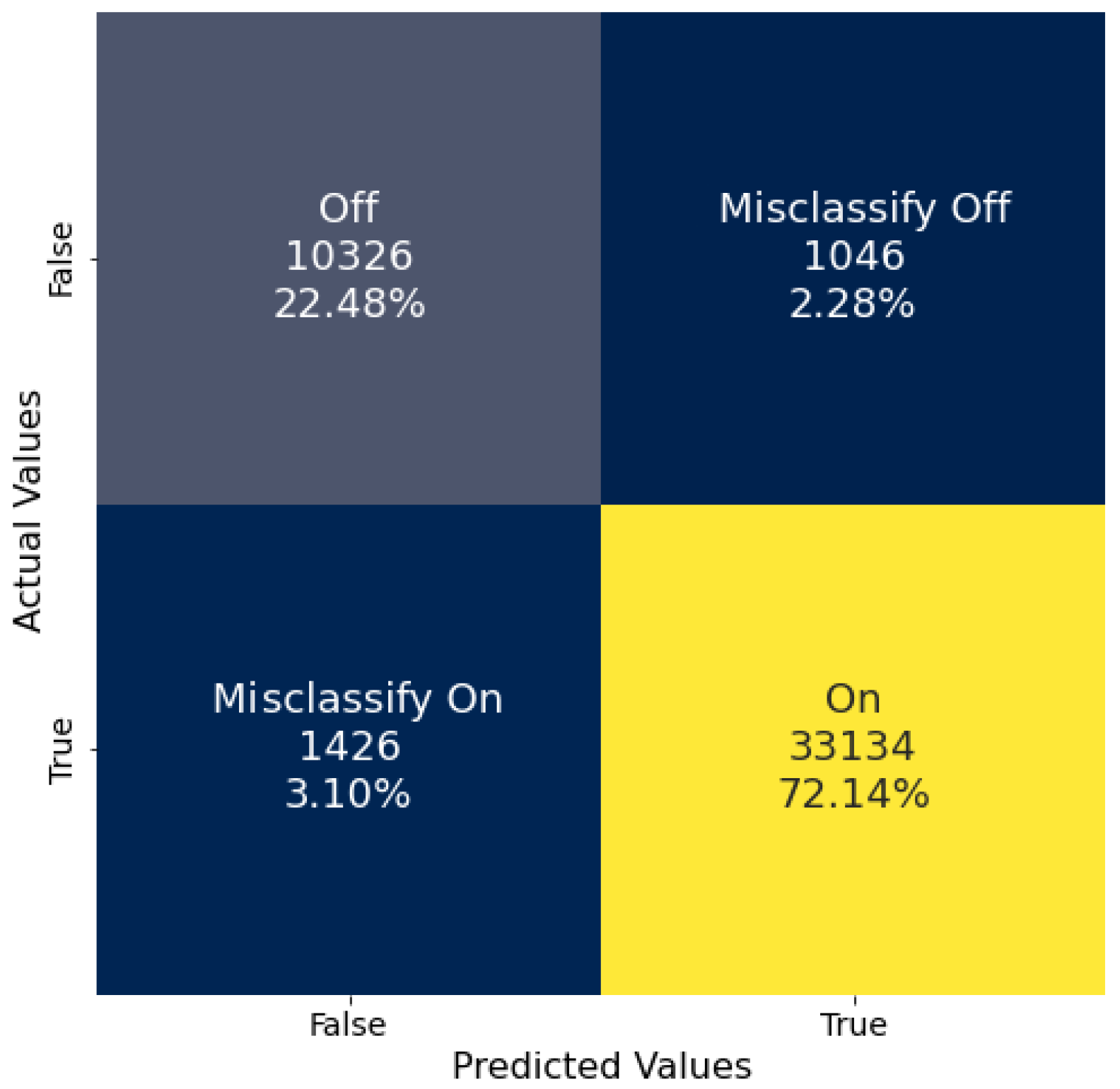
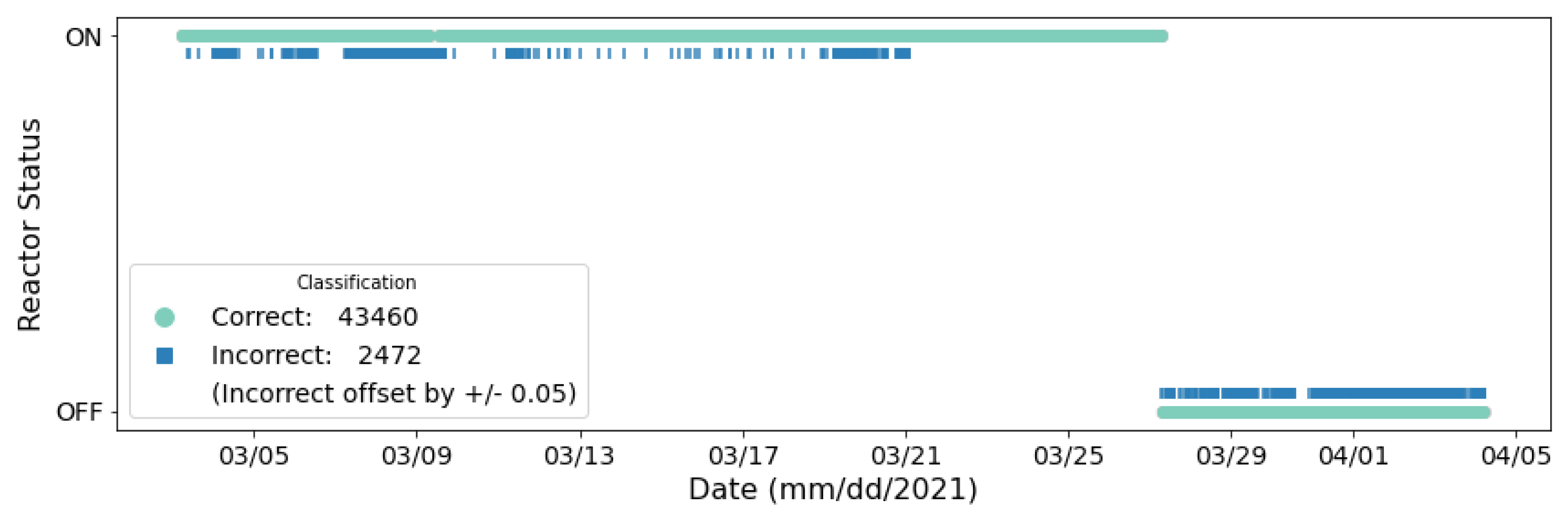
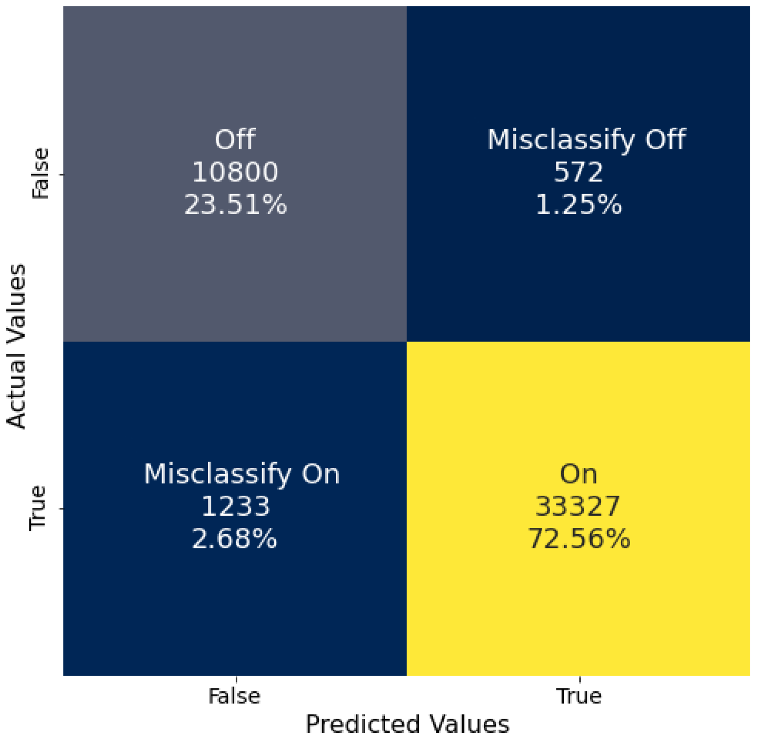
Both of the models tested in this work, a random forest and a DNN, were trained and tested on the same data to enable direct comparison of their performances. The data analyzed were collected from sensor position 9, Figure 1, located next to the cooling fans supporting the HFIR. However, while the duty cycle and variable speed of the fans is related to the status of the reactor, the ML and DL training process used the ON/OFF status labels of the reactor not the fans. Both ML and DL models show a remarkable ability to correctly classify the HFIR operational status. The DNN (95.70%) achieved a slightly higher balanced accuracy than the RF (93.34%), suggesting that the DNN was better suited to generalize to the data as it performed slightly better with Cycle 488. The RF struggled more to generalize to the OFF class than the DNN, but differences observed in the classification of the ON class were negligible.

In real use cases, further analysis of the expected small number of incorrectly-classified time segments could provide additional illumination to existing model biases present in these prototypes and lead to opportunities for performance improvement through model redesign. Future exploration using statistical techniques (e.g., training the models with different bootstrapped samples of the data) could be used to characterize the uncertainty present in the model’s performance characterization.

The overall high classification accuracy obtained suggests that ML shows promise for application to signals collected from unattended remote sensors to verify declared activities involving nuclear reactors. This conclusion is consistent with results published previously [9,10,11]. However, the current study reveals that when converted to frequency space, the signal detected by the 3-axis magnetometers placed near the HFIR cooling fans can be used to classify the reactor operational state more accurately than the time series data [9]. Additionally, a comparable balanced classification accuracy was obtained in this study to that reported by Chai et al. [10]. This indicates that a judiciously placed magnetic field sensor can provide a similar level of declarations verification as does data fusion applied to a single seismo-acoustic station.

The operational cycle of a nuclear reactor used for commercial power production is expected to be dramatically different from that of a nuclear reactor used for plutonium production. This study demonstrates the viability of an important new technique for nuclear treaty monitoring because high fidelity classification tools can be used to independently verify declared operations. Independent verification of declared activities via multiple phenomenologies strengthens monitoring robustness making illicit proliferation activities more difficult to mask.

5. Summary, Conclusions, and Outlook

With the increasing simplicity of nuclear proliferation as science and technology advance, the opportunity arises for treaty verification to grow and develop. Treaty verification plays an important role in slowing the proliferation of nuclear weapons because it acts as a deterrent force. The analysis methodology presented in this paper relies on the availability of passive persistent sensing exterior to a nuclear reactor. This modality of data collection is ideal for nuclear treaty monitoring because it requires no access to the interior of a facility yet provides continuous observation. This study provides a first look at the feasibility of applying machine learning and deep learning techniques to magnetic field sensor data transformed to the frequency domain to verify the declared operational state of a nuclear reactor. The high level of classification accuracy achieved in this study for both ML and DL approaches demonstrates a proof of principle success in applying advanced data analytical techniques to remote sensor data collected exterior to a nuclear reactor.

Future work will examine the transferability of the tuned models to alternate reactors and sites with no additional model changes or training. This will require labeled data be available for those alternate locations so that the generalizability of the trained models can be quantified. Quantification of generalizability will inform the user of existing limitations associated with each trained model.

Other considerations for future studies include utilizing training data that covers a complete calendar year to account for greater variability in the background temperature against which the reactor and cooling fans must operate. This has the potential to produce a more robust model. Additional studies should examine the sensitivity of the classification method to the reactor power ON/OFF threshold value of $7\%$ set by the data owners. Finally, while binary classification provides a foundation, information is available for intermediate power levels between the ON and OFF states. The ability to utilize ML and DL to classify the power levels of this reactor should be investigated.

References

1. Davenport, K. Nuclear Weapons: Who Has What at a Glance. 2022. Available online: https://www.armscontrol.org/factsheets/Nuclearweaponswhohaswhat (accessed on 24 October 2022).
2. Treaty on the Non-Proliferation of Nuclear Weapons; United Nations: New York, NY, USA, 1968.
3. Johnson, R. Unfinished Business: The Negotiation of the CTBT and the End of Nuclear Testing; United Nations Institute for Disarmament Research: Geneva, Switzerland, 2009. [Google Scholar]
4. IAEA. IAEA Safeguards Overview|Factsheet. Available online: https://www.iaea.org/publications/factsheets/iaea-safeguards-overview (accessed on 16 May 2023).
5. Cárdenas, E.; Garcés, M.; Krebs, J.; Watson, S.; Johnson, J.; Hix, J.; Chichester, D. Persistent Acoustic Sensing for Monitoring a Reactor Facility; Virtual [Online]; Institute of Nuclear Materials Management (INNM): Mount Laurel, NJ, USA, 2021; pp. 1–9. [Google Scholar]
6. Cárdenas, E.S.; Takazawa, S.K.; Garcés, M.A.; Chichester, D.L.; Hunley, R.D.; Young, C.D. An Assessment of Persistent Acoustic Monitoring of a Nuclear Reactor during Full Power Generation. Acoustics 2023, 5, 429–443. [Google Scholar] [CrossRef]
7. Gastelum, Z.N.; Goldblum, B.; Shead, T.; Luttman, A. Integrating Physical and Informational Sensing to Support Nonproliferation Assessments of Nuclear-Related Facilities; Technical report SAND2019-7383C; Sandia National Lab. (SNL-NM): Albuquerque, NM, USA, 2019.
8. Eaton, S.W.; Cárdenas, E.S.; Hix, J.D.; Johnson, J.T.; Watson, S.M.; Chichester, D.L.; Garcés, M.A.; Magaña-Zook, S.A.; Maceira, M.; Marcillo, O.E.; et al. An algorithmic approach to predicting mechanical draft cooling tower fan speeds from infrasound signals. Appl. Acoust. 2022, 199, 109015. [Google Scholar] [CrossRef]
9. Tibbetts, J.; Goldblum, B.L.; Stewart, C.; Hashemizadeh, A. Classification of Nuclear Reactor Operations Using Spatial Importance and Multisensor Networks. J. Nucl. Eng. 2022, 3, 243–262. [Google Scholar] [CrossRef]
10. Chai, C.; Ramirez, C.; Maceira, M.; Marcillo, O. Monitoring Operational States of a Nuclear Reactor Using Seismoacoustic Signatures and Machine Learning. Seismol. Res. Lett. 2022, 93, 1660–1672. [Google Scholar] [CrossRef]
11. Rao, N.S.V.; Greulich, C.; Sen, S.; Dayman, K.J.; Hite, J.; Ray, W.; Hale, R.; Nicholson, A.D.; Johnson, J.; Hunley, R.D.; et al. Reactor Power Level Estimation by Fusing Multi-Modal Sensor Measurements. In Proceedings of the 2020 IEEE 23rd International Conference on Information Fusion (FUSION), Rustenburg, South Africa, 6–9 July 2020; pp. 1–8. [Google Scholar] [CrossRef]
12. Calivá, F.; Ribeiro, F.S.D.; Mylonakis, A.; Demazière, C.; Vinai, P.; Leontidis, G.; Kollias, S. A Deep Learning Approach to Anomaly Detection in Nuclear Reactors. In Proceedings of the International Joint Conference on Neural Networks, Rio de Janeiro, Brazil, 8–13 July 2018. [Google Scholar] [CrossRef]
13. Zhong, X.; Ban, H. Pre-trained network-based transfer learning: A small-sample machine learning approach to nuclear power plant classification problem. Ann. Nucl. Energy 2022, 175, 109201. [Google Scholar] [CrossRef]
14. scipy.signal.stft—SciPy v1.8.1 Manual. Available online: https://docs.scipy.org/doc/scipy/reference/generated/scipy.signal.stft.html (accessed on 17 August 2022).
15. Allen, J.B. Short Term Spectral Analysis, Synthesis, and Modification by Discrete Fourier Transform. IEEE Trans. Acoust. Speech Signal Process. 1977, 25, 235–238. [Google Scholar] [CrossRef]
16. Pedregosa, F.; Varoquaux, G.; Gramfort, A.; Michel, V.; Thirion, B.; Grisel, O.; Blondel, M.; Prettenhofer, P.; Weiss, R.; Dubourg, V.; et al. Scikit-learn: Machine Learning in Python. J. Mach. Learn. Res. 2011, 12, 2825–2830. [Google Scholar]
17. Abadi, M.; Agarwal, A.; Barham, P.; Brevdo, E.; Chen, Z.; Citro, C.; Corrado, G.S.; Davis, A.; Dean, J.; Devin, M.; et al. TensorFlow: Large-Scale Machine Learning on Heterogeneous Systems; 2015; Available online: https://www.tensorflow.org/ (accessed on 14 November 2023).
18. Keras. 2015. Available online: https://github.com/fchollet/keras (accessed on 14 November 2023).
19. James, G.; Witten, D.; Hastie, T.; Tibshirani, R. An Introduction to Statistical Learning: With Applications in R, 2nd ed.; Springer: New York, NY, USA, 2017. [Google Scholar]
20. Grandini, M.; Bagli, E.; Visani, G. Metrics for multi-class classification: An overview. arXiv 2020, arXiv:2008.05756. [Google Scholar]
21. Goodfellow, I.; Bengio, Y.; Courville, A. Deep Learning; The MIT Press: Cambridge, MA, USA, 2017. [Google Scholar]
Figure 1. Colored circles indicate positions of the sensors around the High Flux Isotope Reactor (HFIR) at Oak Ridge National Laboratory. A total of 12 sensors are available, but this research focused on the sensor highlighted in the orange circle, number 9. This location was chosen due to its proximity to the cooling fans, shown in the red box, which give off a magnetic field, the chosen sensing modality. Adapted from Ref. [9].
Jne 04 00045 g001
Figure 2. Confusion matrix of the RF model on the data from Cycle 488. On is represented by True and Off is represented by False. The combined 5.38% misclassification value indicates the high accuracy obtained by this model.
Jne 04 00045 g002
Figure 3. RF results for cycle 488 as a function of time. Each marker corresponds to one minute of data. Visual inspection indicates no obvious pattern to the incorrect (misclassified) instances.
Jne 04 00045 g003
Figure 4. Confusion matrix of the DNN model on the data from Cycle 488. On is represented by True and Off is represented by False. The low 3.93% combined misclassification rate indicates the DNN accurately predicts the reactor state.
Jne 04 00045 g004
Figure 5. DNN results for cycle 488 as a function of time. Each marker corresponds to one minute of timeseries data. Visual inspection indicates no obvious pattern to the incorrect (misclassified) instances.
Jne 04 00045 g005