1. Introduction
Coarse Mesh Finite Difference (CMFD) is a widely-used iterative acceleration method for nuclear reactor simulations. CMFD was originally developed for nodal diffusion problems [
1] and later became the method of choice for acceleration of transport problems [
2]. Due to its natural application to eigenvalue problems, CMFD is preferred to other acceleration schemes, such as Diffusion Synthetic Acceleration (DSA) [
3,
4]. Additionally, CMFD introduces a second “coarse” spatial mesh for a homogenized problem. This is in contrast to typical Nonlinear Diffusion Acceleration (NDA) or DSA formulations that only consider a single spatial mesh.
For most problems, CMFD converges reliably and efficiently, provided that the coarse spatial cells are not optically thick. The convergence rate of CMFD was characterized by a Fourier analysis; it is well known that this rate slows and eventually becomes unstable as the optical thickness of the coarse spatial cells increases. We refer to these stability degradation properties of CMFD as linear instability. To emphasize: this type of linear instability can be predicted by linearizing the problem and performing a Fourier analysis on the resulting system of equations.
Unfortunately, CMFD is occasionally affected by another kind of instability, which we call nonlinear instability. This instability occurs in CMFD (and NDA) because artificial nonlinearities are introduced in these methods to maintain equivalence between the discrete low-order diffusion equation and the discrete high-order transport equation. For certain problems in which an estimated value of a coarse-mesh scalar flux quantity is sufficiently small, the estimated value of a nonlinear term can become extremely large (or infinite), leading to extreme numerical fluctuations. When this happens, the normally-stable iterative process is disrupted and can become more slowly convergent or even unstable.
To contend with this, an alternative acceleration scheme, called
Linear Diffusion Acceleration (LDA), was formulated, containing no local nonlinearities. In 1982, an unnamed transport acceleration method was proposed that contains the underlying ideas of LDA [
5]. This method included (i) the use of additive (not multiplicative) terms in the low-order diffusion equations, and (ii) for eigenvalue problems, a solvability condition to ensure that a solution exists to the system of low-order equations. The new LDA method generalizes the earlier method to problems with different spatial meshes for the low-order and high-order equations, and includes linear correction terms to account for the use of linear coarse-mesh quantities. Recent work on these ideas led to the
Semilinear Diffusion Acceleration (SDA) method, a precursor to LDA [
6]. (SDA contains no local nonlinearities for problems in which the low-order and high-order spatial meshes are the same; however, SDA does contain local nonlinearities for problems in which a coarse mesh is employed for the low-order problem). SDA resembles LDA, but it lacks the aforementioned
linear extension to coarse-mesh applications. We consider LDA to be a successor to SDA, in which the coarse-mesh implementation is fully linearized and local nonlinear terms are entirely eliminated. We have submitted a conference paper summarizing the Fourier analysis of LDA [
7]; the details of that work and the present paper (and much more) are presented in the recent PhD thesis of the first author (Z.D.) [
8]. In this thesis, theoretical and numerical results are fully developed for fixed-source and eigenvalue problems, in 1D and multidimensional geometries.
In [
8], LDA was shown to have similar linear stability properties to CMFD for practical problems. Because LDA has no artificial nonlinear terms, it is insensitive to the presence of negative scalar fluxes that might occur anywhere in the problem phase space. In the present paper, we construct problems that demonstrate the vulnerability of CMFD to the presence of very small or negative scalar flux values. For the same problems, we show that LDA converges at the rate predicted by the linearized Fourier analysis. These results show that LDA is unaffected by (i) the occurrence of small or negative scalar fluxes, and (ii) the nonlinear instabilities that occasionally disrupt CMFD-accelerated transport calculations.
The remainder of this paper is organized as follows.
Section 2 briefly describes the fixed-source, one group, 1D CMFD and LDA equations.
Section 3 discusses the nonlinear quantities in the CMFD formulation that can lead to instability in iterations.
Section 4 presents the numerical results, obtained by a 1D S
n test code of case studies that mirror the scenarios outlined in
Section 3. The paper concludes in
Section 5 with a brief discussion.
2. Review of CMFD and LDA Equations
This section provides a brief overview of the CMFD and LDA equations for 1D, fixed-source problems. Detailed information regarding each acceleration method can be found in [
8].
2.1. CMFD Equation
Equation (
1) describes, for a fixed-source problem, the low-order equation to be solved during the CMFD acceleration portion of each outer iteration. The
convention indicates that a quantity
is computed, using
as the weighting function. Traditionally, this is the scalar flux. Spatial discretization is omitted for brevity.
is the scalar flux computed from the transport sweep, and
is the coarse-mesh scalar flux to be computed with the low order system.
D is the diffusion coefficient,
is the nonlinear current coupling coefficient, and
Q is the fixed source. For eigenvalue problems, an inner iteration loop is required to converge the solution to the CMFD equation. Typically, power iteration is used to converge the transport eigenvalue and coarse-mesh scalar flux.
We note that the nonlinear term
(where the coarse-mesh quantity
is the homogenized transport scalar flux), which is estimated using the previous transport sweep, is problematic if an estimate for
is used that is small or negative. This is one source of the nonlinear instabilities that can occur with CMFD. The term
ensures consistency between the scalar flux solutions of the high-order transport equation and the low-order diffusion equation. In Equations (
1) and (
2), the consistency term is
nonlinear and
multiplicative.
2.2. LDA Equation
Equation (
3) describes, for the same fixed-source problem, the diffusion equation to be solved for the low-order LDA calculation. In this equation, the left-hand-side operator contains quantities that are weighted by the initial guess for the fine-mesh scalar flux
. This chosen guess must be globally positive to ensure stability. If a flat guess is chosen, the quantities are volume averaged.
is the neutron current computed from the transport sweep.
The extra terms on the right-hand-side of the LDA equation account for the use of Fick’s law to approximate neutron streaming and the use of cross sections weighted with the initial guess vector. If the initial guess is chosen such that it resembles the converged scalar flux solution, the magnitude of the “lagged” terms on the right-hand-side are reduced, compared to the case in which the initial guess less resembles the converged solution, ultimately resulting in an improved convergence rate. For fission source problems, the LDA equations form a non-standard eigenvalue problem, which requires the use of a different inner iteration loop than power iteration (see [
8] for details on the implementation of LDA for eigenvalue problems). The Fredholm Alternative Theorem is employed to solve this non-standard system [
9].
We note that Equation (
3) contains no artificial nonlinear terms, such as
in Equations (
1) and (
2). The terms on the right-hand side of Equation (
3) that ensure consistency between the scalar flux solutions of the high-order transport equation and the low-order diffusion equation are
linear and
additive.
3. Causes of Numerical Instability in CMFD
In this section, we outline the equations in CMFD that contain nonlinearities with respect to the scalar flux. Such quantities have the potential to become numerically unstable. In
Section 4, these instabilities are demonstrated for contrived problems; LDA is presented alongside CMFD and is shown to be stable.
3.1. Causes of Negative Scalar Flux Quantities
In many transport simulations, the possibility of negative source terms—with resulting nearly zero or negative scalar fluxes—exists, even though the exact solution of the neutron transport equation is guaranteed to be positive. For example, finite element or characteristic methods in which the source is approximated as a linear (or higher-order) function of space in each spatial cell can have approximate source representations that “tilt” negative in part or all of a spatial cell. When this happens, the resulting angular and scalar fluxes can become nearly zero or negative.
Additionally, in the 2D/1D transport formulation in which separate discretizations are used in the radial and axial directions, negative sources can exist, due to the coupling of the transverse leakage terms [
10,
11,
12]. If a spatial region does not contain a fission source, and if the leakage from that region is large, the source can become negative. This is typically addressed through approximations, to ensure positivity of the source, but this usually degrades the accuracy of the calculation [
12,
13].
Generally, the most accurate computational methods for solving neutron transport problems do not guarantee the positivity of the final solution. Certain computational methods (such as the Step and Step Characteristic methods for the linear Boltzmann equation) do guarantee positivity, but these are less accurate than other methods that do not [
14].
3.2. Potential Failure Modes of CMFD
In this section, the 1D numerical formulations of each quantity are given for simplicity and clarity. A finite difference scheme is assumed.
3.2.1. Numerical Diffusion Coefficient
The traditional expression for the numerical diffusion coefficient used in Fick’s Law is presented in Equation (
4). In this expression,
is the coarse cell homogenized total macroscopic cross section in coarse cell
k, and
is the width of coarse cell
k.
is the fine-mesh scalar flux in fine cell
j.
The expression for possesses the potential for numerical instability in the denominator term. If can be negative, the terms and have the potential to be equal in magnitude and opposite in sign. Since is a flux-weighted average over a coarse cell, there is a possibility that the presence of negative scalar flux quantities can result in a negative cross section. If the two denominator terms are nearly equal in magnitude and opposite in sign, the denominator of approaches zero. Additionally, in near-void regions with extremely small optical thicknesses, the denominator also approaches zero. In either case, small floating point errors can be greatly magnified, is unbounded, and the numerical stability is compromised.
3.2.2. Nonlinear Current Coupling Coefficient
The transport correction term, or nonlinear current coupling coefficient, typically referred to as
, is defined in Equation (
5). In this expression,
is the neutron current at the interface of coarse cells
k and
.
is defined in Equation (
4).
is the volume-averaged scalar flux in coarse cell
k.
possesses the potential for numerical instability in two ways:
The first is due to the presence of in the numerator. If becomes unstable, will as well.
If the coarse cell scalar flux in two adjacent cells are equal in magnitude and opposite in sign, or otherwise evaluate near zero, the denominator in can become extremely close to, or equal to, zero.
3.2.3. Prolongation of the Scalar Flux
The prolongation equation for updating the fine-mesh scalar flux using the most recent coarse-mesh scalar flux solution is shown in Equation (
6). In this expression,
is the scalar flux in fine cell
j. Coarse cell
k is a contiguous union of fine cells, each of which is scaled by a multiplicative factor. Outer iteration superscripts are included in this expression, denoted by
ℓ. The update scheme is implementation-dependent, so in this example, the transport sweep is assumed to take place before the acceleration step. We note that other prolongation operators have been developed that are linear [
15], but a multiplicative update is generally used.
is the scalar flux obtained from the transport sweep,
is the homogenized scalar flux from the transport sweep,
is the solution from the acceleration step, and
is the scalar flux to be used in the source for the transport sweep in the next iteration.
If the scalar flux in a single coarse cell region approaches zero, the update ratio for the fine-mesh scalar flux can become sensitive to small fluctuations. In this case, the fine-mesh scalar flux can become unstable.
4. Case Studies of the Numerical Instability of CMFD
Here, we present three case studies that are paired with the proposed failure modes of CMFD described in
Section 3.2. Each of these cases is a contrived problem designed to demonstrate the susceptibility of a numerical implementation of CMFD to numerical instability. The contrived problems involve a fixed-source problem in which, in a single fine spatial cell, the internal source is taken to be negative. (Elsewhere in the system, the internal source is positive.) By adjusting the magnitude of the single-cell negative source, the scalar flux in that cell can be driven to be zero (and negative). This can lead to different types of nonlinear CMFD failure modes. For each case, a range of configurations is investigated. Within this range, CMFD transitions from stable to unstable. The numbers of outer iterations required for convergence with CMFD and LDA are plotted, as well as the quantity that results in instability for CMFD.
Accelerated S16 fixed-source transport problems are investigated here, with the diamond-difference spatial discretization. In each of the three studies, a 1D problem with 10 fine spatial mesh cells, each of width 0.1 cm is considered. The total width of the slab is 1.0 cm, and vacuum boundary conditions are imposed on both sides of the system. Unless otherwise stated, the internal source magnitude and total cross section are equal to unity. Each coarse spatial cell contains two fine cells. Thus, the system has five coarse cells, each of width 0.2 cm. A cap of 1000 outer iterations is imposed, with iterations halted when this limit is exceeded. Simulations that reach this threshold are considered to be divergent.
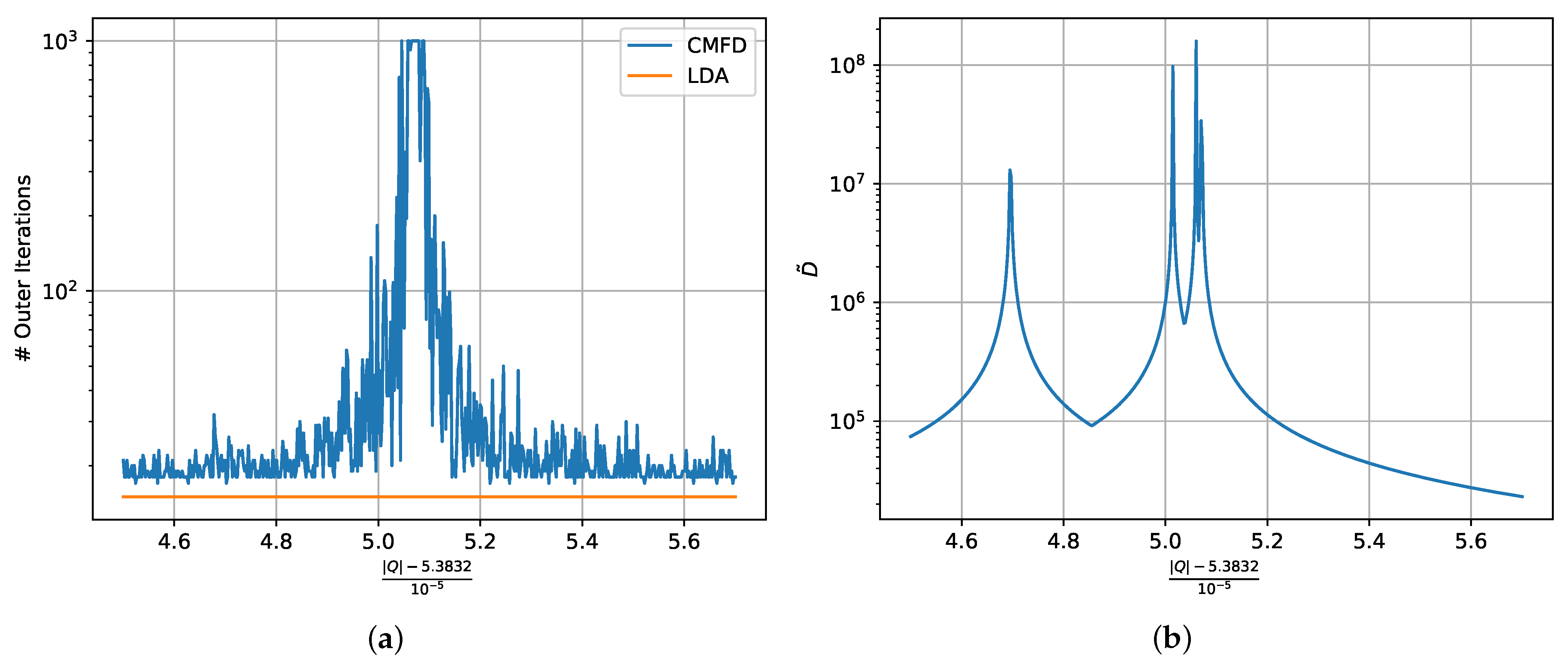
4.1. Instability Due to the Numerical Diffusion Coefficient
In this case, the value of the source in the 7th fine spatial cell from the left side of the geometry is varied over a range of negative values. Additionally, the magnitude of
in the 7th fine cell is taken to be a factor of 10 greater than that in the other cells. At a critical value of the negative source, the flux weighted total cross section for the fourth coarse cell becomes opposite in sign and equal in magnitude to the total cross section of the coarse cell to the right. In this case, the value of
at the interface of these cells becomes unstable, leading to divergence with CMFD.
Figure 1a shows the number of outer iterations required for convergence as a function of the negative source magnitude in the 7th fine cell for both CMFD and LDA. Because LDA uses volume-weighted cross sections, with correction terms in the source to account for error due to the lack of applying the scalar flux weight, it remains stable.
Figure 1b shows the magnitude of
at the cell interface when using CMFD. It is evident that
becomes very large in the region where CMFD diverges.
Figure 1a,b also shows that the performance of the LDA method is unaffected by the existence of the negative scalar fluxes.
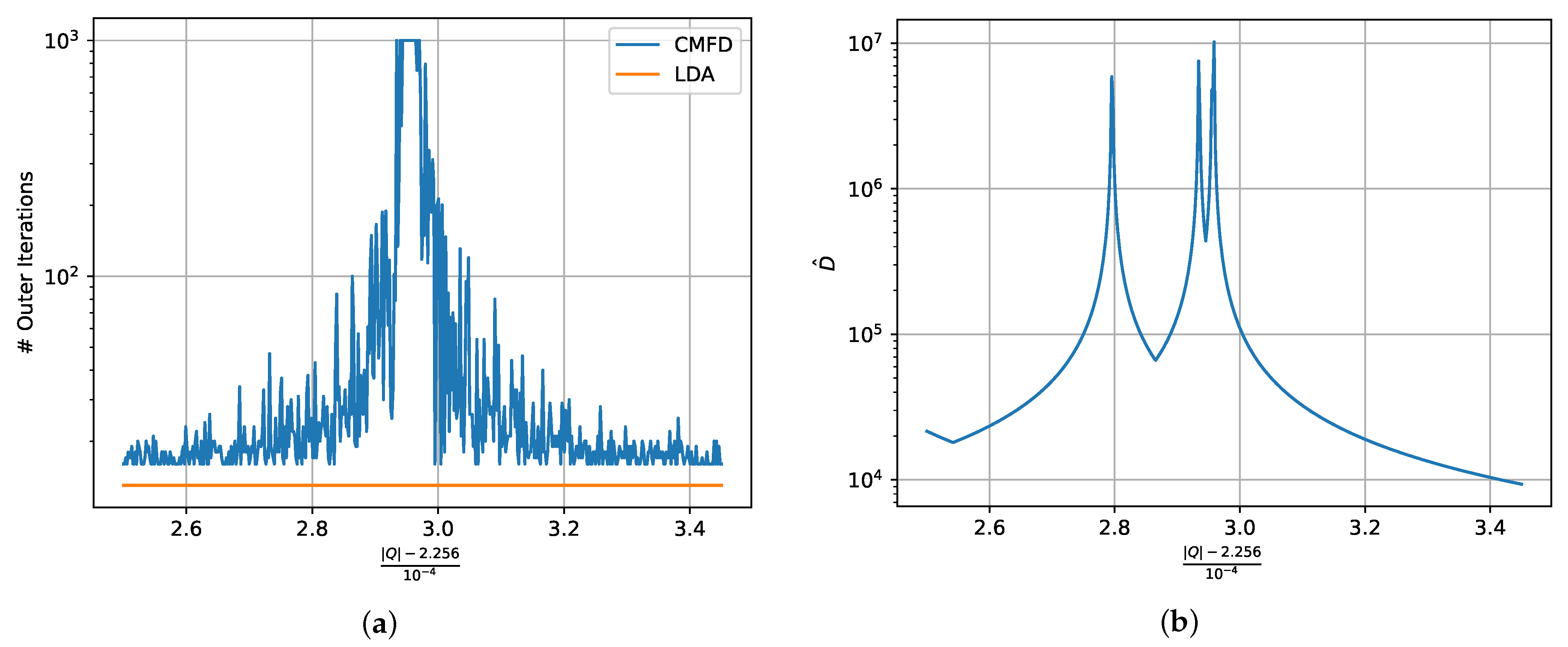
4.2. Instability Due to the Nonlinear Current Coupling Coefficient
For this study, the negative source magnitude is adjusted to result in CMFD failure due to instability in the
quantity. A critical value of the negative source results in the coarse-cell scalar flux for the 4th and 5th coarse cell becoming opposite in sign and equal in magnitude. CMFD is seen to diverge once the two quantities are sufficiently close, as shown in
Figure 2a. LDA does not require
in its formulation, and therefore it remains stable.
Figure 2b shows the magnitude of
at the interface of the 4th and 5th coarse cells. It is evident that
becomes large in the region where CMFD diverges.
Figure 2a,b shows that, as before, the performance of the LDA method is unaffected by the existence of negative scalar fluxes.
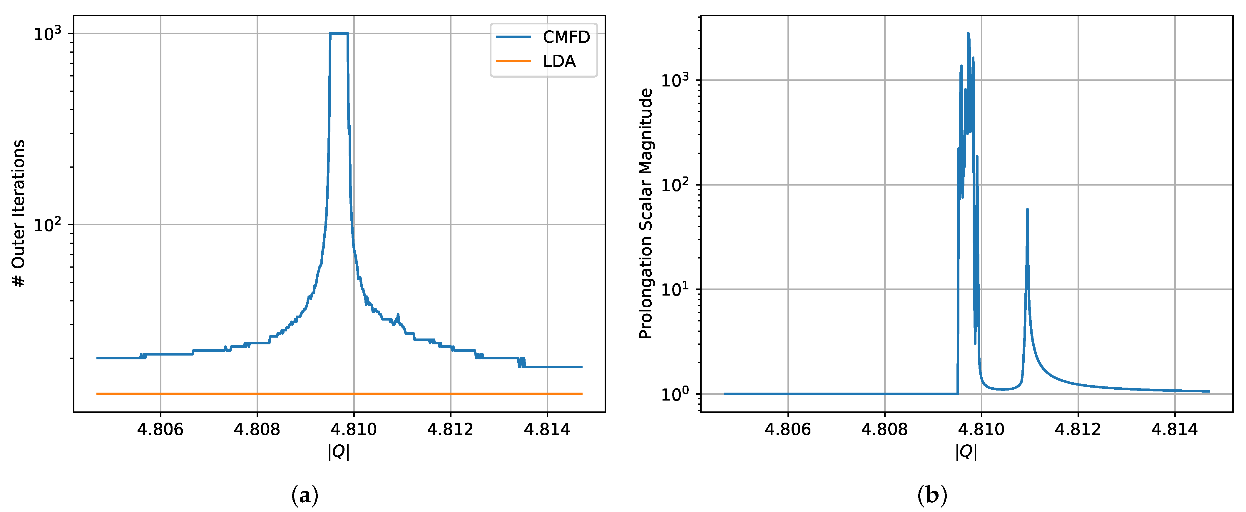
4.3. Instability Due to the Prolongation of the Scalar Flux
This section focuses on the multiplicative prolongation scalar that is used to update the fine-mesh scalar flux once the low order problem has been solved. Equation (
7) defines the multiplicative scalar, which consists of the ratio of the newly-computed coarse-mesh scalar flux to that from the previous iteration.
If the scalar flux in a coarse-mesh cell becomes small, this quantity can become unstable as shown in
Figure 3a.
Figure 3b shows the magnitude of
, which becomes large in the region where CMFD is unstable. Because prolongation in LDA is done in an additive manner, this instability cannot occur.
Figure 3a,b shows that, once again, the performance of the LDA method is unaffected by the existence of negative scalar fluxes.
5. Conclusions
Potential failure modes of CMFD arise from nonlinear quantities that are present in the numerical implementation. LDA, which was specifically formulated to avoid these nonlinearities, is not susceptible to related numerical instabilities. In each of the three case studies, CMFD was shown to diverge within a critical range. It should be noted that in the region near the point of divergence for CMFD, the number of iterations required for convergence dramatically increased. Thus, if a quantity in the numerical CMFD formulation nears a “critical point,” the overall iteration scheme can exhibit a severe performance penalty.
The problems in this study were deliberately designed with a negative source in one cell to yield a nearly zero or negative scalar flux in the same cell. These problems are contrived—they would probably never be considered in a practical application. However, situations occur in practical multidimensional problems in which, due to truncation or modeling errors, negative fluxes can occasionally occur. The work presented in this paper studies the behavior of CMFD and LDA when negative scalar fluxes occur under controlled circumstances in which the location of the negative scalar flux can be predicted.
Our results are not surprising. They demonstrate that CMFD can degrade or even fail in the presence of negative scalar fluxes, while LDA does not fail. For problems in which negative scalar fluxes do not occur, even while converging toward a positive solution, CMFD and LDA will have similar convergence properties. However, this is not the case for problems in which negative scalar fluxes can occur. For such problems, our work shows that LDA is a more robust alternative to CMFD. Alternatively, the work in this paper demonstrates that CMFD is susceptible to nonlinear instabilities, while LDA is not susceptible to these instabilities.
This work will hopefully improve the understanding of why CMFD can degrade (or fail) in certain (presumably rare) problems. We also hope that this work will influence ongoing research involving CMFD applied to the approximate 2D–1D method, which does not guarantee positive solutions.
Author Contributions
Conceptualization, Z.D., B.K. and E.L.; methodology, Z.D., B.K. and E.L.; software, Z.D.; validation, Z.D.; formal analysis, Z.D., B.K. and E.L.; investigation, Z.D.; resources, B.K.; data curation, Z.D.; writing—original draft preparation, Z.D.; writing—review and editing, Z.D., B.K. and E.L.; visualization, Z.D.; supervision, B.K. and E.L.; project administration, B.K. and E.L.; funding acquisition, B.K. All authors have read and agreed to the published version of the manuscript.
Funding
This research was supported by the Consortium for Advanced Simulation of Light Water Reactors (
www.casl.gov), an Energy Innovation Hub (
http://www.energy.gov/hubs) for Modeling and Simulation of Nuclear Reactors under U.S. Department of Energy Contract No. DE-AC05-00OR22725. Additionally, this research was conducted with the support of the Rackham Merit Fellowship at the University of Michigan.
Data Availability Statement
Not applicable.
Conflicts of Interest
The authors declare no conflict of interest. The funders had no role in the design of the study; in the collection, analyses, or interpretation of data; in the writing of the manuscript, or in the decision to publish the results.
References
- Smith, K. Nodal method storage reduction by nonlinear iteration. Trans. Am. Nucl. Soc. 1983, 44, 265–266. [Google Scholar]
- Smith, K.; Rhodes, J. Full-Core, 2-D, LWR Core Calculations with CASMO-4E. In Proceedings of the PHYSOR 2002—International Conference on the New Frontiers of Nuclear Technology: Reactor Physics, Safety and High-Performance Computing, Seoul, Korea, 7–10 October 2002. [Google Scholar] [CrossRef]
- Kopp, H.J. Synthetic Method Solution of the Transport Equation. Nucl. Sci. Eng. 1963, 17, 65–74. [Google Scholar] [CrossRef]
- Gelbard, E.M.; Hageman, L.A. The Synthetic Method as Applied to the Sn Equations. Nucl. Sci. Eng. 1969, 37, 288–298. [Google Scholar] [CrossRef]
- Gelbard, E.M.; Adams, C.H.; McCoy, D.R.; Larsen, E.W. Acceleration of Transport Eigenvalue Problems. Trans. Am. Nucl. Soc. 1982, 41, 309–310. [Google Scholar]
- Dodson, Z.; Adamowicz, N.; Kochunas, B.; Larsen, E. SDA: A Semilinear CMFD-Like Transport Acceleration Scheme without D-Hat. In Proceedings of the M&C 2019-International Conference on Mathematics & Computational Methods Applied to Nuclear Science & Engineering, Portland, OR, USA, 25–29 August 2019. [Google Scholar]
- Dodson, Z.; Kochunas, B.; Larsen, E. Fourier Analysis of Coarse Mesh Finite Difference and Linear Diffusion Acceleration for Spatially Heterogeneous Systems. In Proceedings of the M&C 2021-International Conference on Mathematics & Computational Methods Applied to Nuclear Science & Engineering, Virtual Meeting, 3–7 October 2021. [Google Scholar]
- Dodson, Z. Linear Diffusion Acceleration for Neutron Transport Problems. Ph.D. Thesis, University of Michigan, Ann Arbor, MI, USA, 2021. [Google Scholar]
- Ramm, A.G. A simple proof of the Fredholm alternative and a characterization of the Fredholm operators. Am. Math. Mon. 2001, 108, 855–860. [Google Scholar] [CrossRef]
- Joo, H.G.; Cho, J.Y.; Kim, K.S.; Lee, C.C.; Zee, S.Q. Methods and performance of a three-dimensional whole-core transport code DeCART. In Proceedings of the PHYSOR 2004: The Physics of Fuel Cycles and Advanced Nuclear Systems-Global Developments, Chicago, IL, USA, 25–29 April 2004; pp. 21–34. [Google Scholar]
- Kelley, B.W.; Larsen, E.W. A consistent 2D/1D approximation to the 3D neutron transport equation. Nucl. Eng. Des. 2015, 295, 598–614. [Google Scholar] [CrossRef] [Green Version]
- Zhao, C.; Liu, Z.; Liang, L.; Chen, J.; Cao, L.; Wu, H. Improved leakage splitting method for the 2D/1D transport calculation. Prog. Nucl. Energy 2018, 105, 202–210. [Google Scholar] [CrossRef]
- Hursin, M. Full Core, Heterogeneous, Time Dependent Neutron Transport Calculations with the 3D Code DeCART. Ph.D. Thesis, University of California at Berkeley, Berkeley, CA, USA, 2010. [Google Scholar]
- Lathrop, K.D. Spatial Differencing of the Transport Equation: Positivity vs. Accuracy. J. Comput. Phys. 1969, 4, 475–498. [Google Scholar] [CrossRef]
- Wang, D.; Xiao, S. A linear prolongation approach to stabilizing CMFD. Nucl. Sci. Eng. 2018, 190, 45–55. [Google Scholar] [CrossRef]
| Publisher’s Note: MDPI stays neutral with regard to jurisdictional claims in published maps and institutional affiliations. |
© 2021 by the authors. Licensee MDPI, Basel, Switzerland. This article is an open access article distributed under the terms and conditions of the Creative Commons Attribution (CC BY) license (https://creativecommons.org/licenses/by/4.0/).


