Spatiotemporal Analysis of Obesity: The Case of Italian Regions

Abstract

This study examines the spatial and temporal evolution of obesity among adults in Italian regions. In Italy, regional administrative areas are responsible for providing health services. Moreover, Italian regions present different socioeconomic conditions and health and nutritional habits. As a result, a regional analysis of the spatiotemporal evolution of obesity allows the identification of key areas for prevention and control, enabling the design of more targeted and effective interventions. In this study, the geographic clustering of obesity in Italy was explored by analyzing the local spatial autocorrelation of regional-level prevalence rates of adulthood obesity between 2010 and 2022, updating and expanding the existing literature. Data from the Health For All repository are analyzed to determine distribution patterns and trends, employing choropleth maps, Moran’s Index and Welch’s t-test. Gender inequalities have been underlined both in the spatial and temporal distribution. Results show that obesity exhibits spatial clustering, with greater severity in the south. During the period under analysis, obesity prevalence rates in Italy show a tendency to grow, with a sharp increase during the COVID-19 lockdown.

1. Introduction

Chronic non-communicable diseases (NCDs) have become a major global public health challenge, with increasing prevalence across various demographic groups. Obesity is among the major risk factors for chronic diseases. It is associated with a range of adverse health outcomes, including cardiovascular diseases, diabetes, and reduced life expectancy, and it is a challenge for health systems [1]. Obesity is recognized as a major public health problem in Europe, where it has reached alarming levels, posing substantial health, social, and economic burdens on European societies: In 2021, approximately 1.1 million deaths in the EU, equivalent to nearly 21% of all deaths, were attributable to the combined impact of smoking, excessive alcohol use and high body-mass index [2]. Even though Italy demonstrates relatively favorable conditions for women, projections suggest an increasing average obesity trend [3]. Furthermore, preventable inequalities in health (including obesity) persist between regions within Italy [4,5,6,7,8].

Understanding the spatial and temporal distribution of obesity is complex due to regional variation and the interplay of individual, contextual, and environmental determinants [9]. Nevertheless, such understanding is essential for designing effective public health interventions aimed at reducing obesity-related health risks.

This study examines trends in regional prevalence of obesity in Italy over a 13-year period (2010–2022) using a spatiotemporal framework, with the aim of providing useful information to implement interventions in more specific areas. The increasing availability of geospatial health data provides an opportunity to analyze obesity patterns beyond simple national averages.

This is a significant enhancement to the usual monitoring of regional-level inequalities in obesity in policy reports [10,11] as it extends the usual approach, employing spatial analysis and testing differences among regions and genders. This is of the utmost importance in Italy, since obesity rates can exhibit significant spatial correlation, influenced by socioeconomic factors, lifestyle behaviors, and regional healthcare policies.

Specifically, this study answers the following research questions:

• Is there a spatial association among Italian regions in obesity prevalence rates? This helps identify similarities among regions in order to design more targeted and specific policies.
• Are these regional associations the same for the two genders?
• Are spatial associations consistent over time, or has there been an evolution in obesity prevalence?

Across Italian regions, there are strong structural differences in general culture, social norms, and economic development [12]. Regional inequalities in excess adiposity are of interest themselves, given the important socio-economic ramifications of obesity and the implied clustering of the health risks and disadvantages at the regional level. They are also important because they may influence resource allocation and to infer the success of area-based policies to tackle obesity. From the perspective of health policy, better understanding of the distribution of regional inequalities in obesity is useful for local authorities, given their enhanced role as leaders for local population health.

The diversity observed among Italian regions may then influence obesity and related phenomena [13]. For this reason, proposing an analysis that takes into account heterogeneity is essential [4]. Furthermore, gender aspects should also be considered, given potential physical and genetic differences as well as cultural ones [1,14].

This research leverages spatial and temporal areal data to investigate obesity patterns across Italy’s 20 administrative regions. We use a dataset from the Health For All (HFA) platform of the Italian National Institute of Statistics (ISTAT).

The spatial distribution and temporal trends of obesity are provided: choropleth maps, time series analyses, and spatial correlation metrics such as Moran’s I are employed to assess clustering and regional disparities. In particular, Moran’s I values quantify the degree of spatial autocorrelation in regional obesity rates across Italian regions. This study offers also an addition to the methods to deal with islands in spatial analysis, considering with particular accuracy tendencies in the two major Italian islands.

The next sections will delve deeper into the methodology, data sources, and analytical techniques employed in this study. Section 3 shows the results of the study, while a discussion and the conclusion are presented at the end of the paper.

2. Materials and Methods

This study provides a comprehensive overview of the spatial and temporal distribution of obesity across Italian regions. The analysis begins by employing choropleth maps to visualize the temporal average obesity rates at the regional level. These maps are further extended to highlight the differences that exist between the two genders.

In addition to spatial representations using maps, bar plots are employed to display the average obesity rates over time, with distinctions made by region and by geographical zones. This allows for a detailed comparison of obesity rates both regionally and across these macro-areas. The distribution of obesity rates through time is further explored through boxplots, illustrating the variation within each macro-area and providing a clearer understanding of regional differences.

To capture temporal trends, time series plots of obesity rates are presented, both for the overall population and disaggregated by sex, across the defined macro-areas. A time series boxplot is also included, offering additional insights into the temporal evolution of obesity rates by macro-area. Furthermore, choropleth maps are used to visualize obesity rates for specific years (2010, 2012, 2014, 2016, 2018 and 2022), highlighting changes in spatial patterns over time.

The second part of this section focuses on spatial correlation, introducing the weights matrix and how it is constructed. This matrix is essential for the spatial smoothing and for the calculation of Moran’s Index (Moran’s I) statistics. Such a measure is helpful for identifying whether obesity rates exhibit spatial dependence, i.e., whether regions with high or low obesity rates tend to cluster geographically. Visualizations of Moran’s I evolution through time and by gender are provided to obtain a picture of the variability of the spatiotemporal trend.

Finally, the paper presents smoothed choropleth maps, derived from the spatial smoothing technique employed.

2.1. Data

This study analyses the obesity prevalence rate registered in each region, and by sex, collected from HFA from 2010 to 2022. Here, the definition of obesity follows the WHO classification [15]: an individual with a Body Mass Index (BMI) greater than or equal to 30 can be classified as with obesity. The longitudinal dataset collects information on the 20 Italian regions from 2010 to 2022 (13 years). The data under study are specifically spatiotemporal areal data, which can be viewed as a collection of time series for each spatial unit. Spatial correlation, if present, depends on the geographical location of the areal units and their neighboring regions, while temporal correlation, if present, depends on time persistency [16,17].

The longitudinal dataset analyzed in this paper has been constructed by extracting information from the Istat Health For All (HFA) platform. The HFA provides a selection of indicators on health, including health services, needs, lifestyles, demographics, social, economic and environmental contexts, basic demographic data, health status and determinants, and healthcare.

Italian regions are divided according to the NUTS 1 classification into 5 different geographical zones: Northwest, Northeast, Centre, South and Islands (

Table 1. Italian regions and their geographical zones ¹.

Geographical Zone	Region
Northwest	Piemonte, Valle d’Aosta, Lombardia, Liguria, Emilia-Romagna
Northeast	Trentino-Alto Adige, Veneto, Friuli-Venezia Giulia
Centre	Toscana, Umbria, Marche, Lazio
South	Abruzzo, Molise, Campania, Puglia, Basilicata, Calabria
Islands	Sicily, Sardinia

¹ Source: https://www.istat.it/classificazione/codici-dei-comuni-delle-province-e-delle-regioni/ (accessed on 8 April 2025).

). This classification corresponds to areas that differ in several social, demographic and economic features.

2.2. Methodology: Spatiotemporal Analysis

In a spatiotemporal context, it is crucial to investigate whether spatial patterns exist across the regions under study, and if so, to assess their strength.

Spatial patterns specifically refer to the tendency of neighboring areal units to exhibit similar values. Such patterns can give rise to complex geographic processes and structures that emerge from local interactions, so that careful consideration is needed when measuring and analyzing relationships between nearby entities [18].

Spatiotemporal analysis is a fundamental approach across various disciplines, particularly in social sciences and public health, since it can uncover significant features such as spatial and temporal patterns, global and local dependence structures, and outliers [19,20]. Social science research needs to explore the integration of spatial and temporal dimensions, highlighting the importance of studying how spatial patterns evolve over time [21,22]. Spatial analysis techniques, including those with temporal extensions, are usefully employed in epidemiology and public health [19,23,24].

Maps offer valuable visualizations during the exploratory stage, facilitating a better understanding of spatial relationships. For areal data, one of the most commonly employed types of maps is the choropleth map [17]. In a choropleth map, each spatial unit (or polygon) is shaded based on the value of the variable being represented, allowing for a clear and intuitive visualization of spatial variations across different areas.

Mapping raw data or indices constructed from them (i.e., temporal averages) is surely an important tool to identify spatiotemporal patterns. However, to enhance the clarity of spatial relationships within the data, it is often beneficial to apply spatial smoothing techniques. While preliminary mapping provides a starting point, smoothing can help to reveal underlying spatial relationships more effectively. Various techniques are available for spatial smoothing, with first-order smoothing being a common approach for areal data [16,17]. This method helps to reduce noise and highlight more significant spatial patterns. More specifically, a first-order smoothed value for area i can be obtained by calculating a weighted average of the value in area i together with the areas neighboring i. This can be done through the use of a “weights matrix” [16,17].

2.3. Statistical Methodology: Moran’s Index

Given the vector of measurements y = (y₁, …, y_N) associated with a set of N areal units, the N × N weights matrix (or “proximity matrix” or “adjacency matrix”) W is such that entries w_ij, i = 1, …, N, j = 1, …, N, spatially connect neighboring units i and j in some way. Neighbors are represented by writing i∼j, where i ≠ j.

Various definitions exist for the weights matrix W and for determining neighboring relationships between areal units. Here, the binary encoding approach is followed, as it is one of the most commonly used for areal data and modelling [16]. Specifically, the entries w_ij in the adjacency matrix are defined such that w_ij = 1 if region i and region j share a common border, and 0 otherwise. This last case includes the diagonals, as a region is not considered its own neighbor (so that w_ii = 0 for all i). In the majority of specifications, including the one employed in this study, the weights matrix W is symmetric. In this study, weights in each row are binary and represent the weights for averaging over neighboring units, so that every region has the same strength of connection [17]. This methodology refers to the main literature on spatial statistics dealing with areal data, and it is the usual method to indicate the fact that areas share a border (w_ij = 1) or not (w_ij = 0) [16,17]. Various definitions exist for the weights matrix W and for determining neighboring relationships between areal units [16,17]. However, alternative methodologies for a weights matrix are less straightforward to interpret and may introduce complexity and potentially obscure results [17].

In order to measure the strength of spatial association among areal units, the Moran’s I index is employed [16]. Among the possible proximity matrices, the binary weights matrix W introduced above is employed to construct those statistics. The Moran’s index I is constructed as follows:

$$I={\displaystyle \frac{N\sum _i\sum _j{w}_{ij}\left(Y_i-\overline{Y}\right)\left(Y_j-\overline{Y}\right)}{\sum _i\sum _j{w}_{ij}\sum _j{\left(Y_j-\overline{Y}\right)}^2}}$$

(1)

where:

-

N is the number of spatial units.

-

Y_i, Y_i are the values of the variable at location or j.

-

$\overline{\mathrm{Y}}$ is the average of the variable.

-

w_ij is the spatial weight between unit i and unit j, indicating the spatial proximity or connection between units i and j.

A positive Moran’s I implies that similar values are spatially clustered (high–high or low–low), while a negative value indicates a checkerboard-like pattern (high–low). A value near zero suggests spatial randomness.

Moran’s index I is not strictly bounded within the interval [−1, 1], although values outside this range can occur only in extreme cases [16].

Though often used descriptively, under the null hypothesis of spatial independence (i.e., no spatial correlation), Moran’s I can also be compared to its expected value and variance (which depend on the structure of W) to assess statistical significance. In order to do that, we employed a non-parametric bootstrap procedure rooted in spatial randomization. Specifically, for each year and sex, we computed the observed Moran’s I statistic and compared it to a reference distribution obtained by permuting the regional obesity values 999 times, thereby simulating the null hypothesis of spatial randomness.

This permutation-based approach generates a null distribution of Moran’s I statistics that retains the observed spatial weights matrix but disrupts the spatial structure of the obesity values. The test assumes exchangeability under the null, which is satisfied by random permutation of the data while keeping the spatial configuration (i.e., the contiguity matrix) fixed. The p-value is computed as the proportion of permuted Moran’s I statistics that are greater than or equal to the observed statistic (i.e., a one-sided test), and the 95% confidence interval is obtained via the empirical 2.5th and 97.5th percentiles of the permutation distribution.

This bootstrap method is robust and distribution-free, avoiding assumptions of normality or parametric forms. This approach is useful for guiding further investigation into underlying regional determinants, policy impacts, or socio-economic disparities. However, due to the stochastic nature of the bootstrap and its dependency on the spatial configuration, it should be interpreted with caution: because the null distribution is derived under the hypothesis of no spatial structure, significant results merely suggest departure from that specific null and do not establish causality or mechanism.

The weights matrix W encodes the spatial structure of the data by formalizing theconcept of “neighboring regions” via the binary weights introduced before, as it is common in areal data, especially when the primary aim is to capture the direct spatial structure [16].

The “spdep” R package is employed for analyzing spatial correlation across regions, using the weights matrix W [25].

2.4. Statistical Methodology: Spatial Smoothing

Regional differences can be sensitive to local variability. Spatial smoothing addresses this by using the structure of W to calculate averaged values that are less sensitive to random variation and more reflective of the underlying spatial structure.

Mapping raw data or indices constructed from them (i.e., temporal averages) is surely an important tool for gaining a first clue of potential spatial (and spatiotemporal) patterns. However, to enhance the clarity of spatial relationships within the data, it is often beneficial to apply spatial smoothing techniques. While preliminary mapping provides a starting point, smoothing can help to reveal underlying spatial relationships more effectively. Various techniques are available for spatial smoothing, with first-order smoothing being a common approach for areal data [16,17]. This method helps to reduce noise and highlight more significant spatial patterns. More specifically, a first-order smoothed value for area i can be obtained by calculating a weighted average of the value in area i together with the neighboring areas to i. This can be done through the use of a “weights matrix”. The weights matrix W can be used to generate smoothed values for the obesity rates. Specifically, for each region i, at year t, a smoothed obesity rate is calculated by averaging the obesity rates of neighboring regions j∼i at the same time t, with neighborhood relationship defined by the binary weights matrix W specified as before (see Section 2.3).

The smoothed value for region i is typically calculated as:

$${\tilde{Y}}_i={\displaystyle \frac{1}{n}}\sum _{j~i}{Y}_j$$

(2)

where the summation is over the neighbors j of i, n_i is the number of such neighbors and j∼i indicates the neighboring relationship, for all j ≠ i, as a region is not considered a neighbor of itself. This local average produces maps that emphasize spatial trends through the neighboring structure.

The use of smoothing is not arbitrary, since it directly reflects the hypothesis behind Moran’s I: that values in neighboring regions may be similar due to latent spatial processes. Thus, smoothing can reinforce the presence of spatial autocorrelation.

Moran’s I provides a quantitative measure of spatial autocorrelation, while smoothing offers a visual representation of it. Used together, they form a coherent strategy for spatial analysis: while Moran’s I confirms whether the spatial patterns seen on the maps are statistically meaningful, smoothed maps enhance the interpretability of those patterns, reducing visual noise and clarifying trends.

This dual approach is particularly important in policy-relevant contexts like obesity analysis: because raw maps might suggest clusters or gradients that could be not systematic, Moran’s I helps assess whether those patterns are non-random, while smoothing helps communicate them more clearly.

3. Results

3.1. Spatial Analysis

There were large differences in obesity rates among the twenty geographic regions of Italy: the map in Figure 1 shows the temporal averages over the period 2010–2022 of the obesity rates, in order to highlight the spatial structure of obesity in Italy.

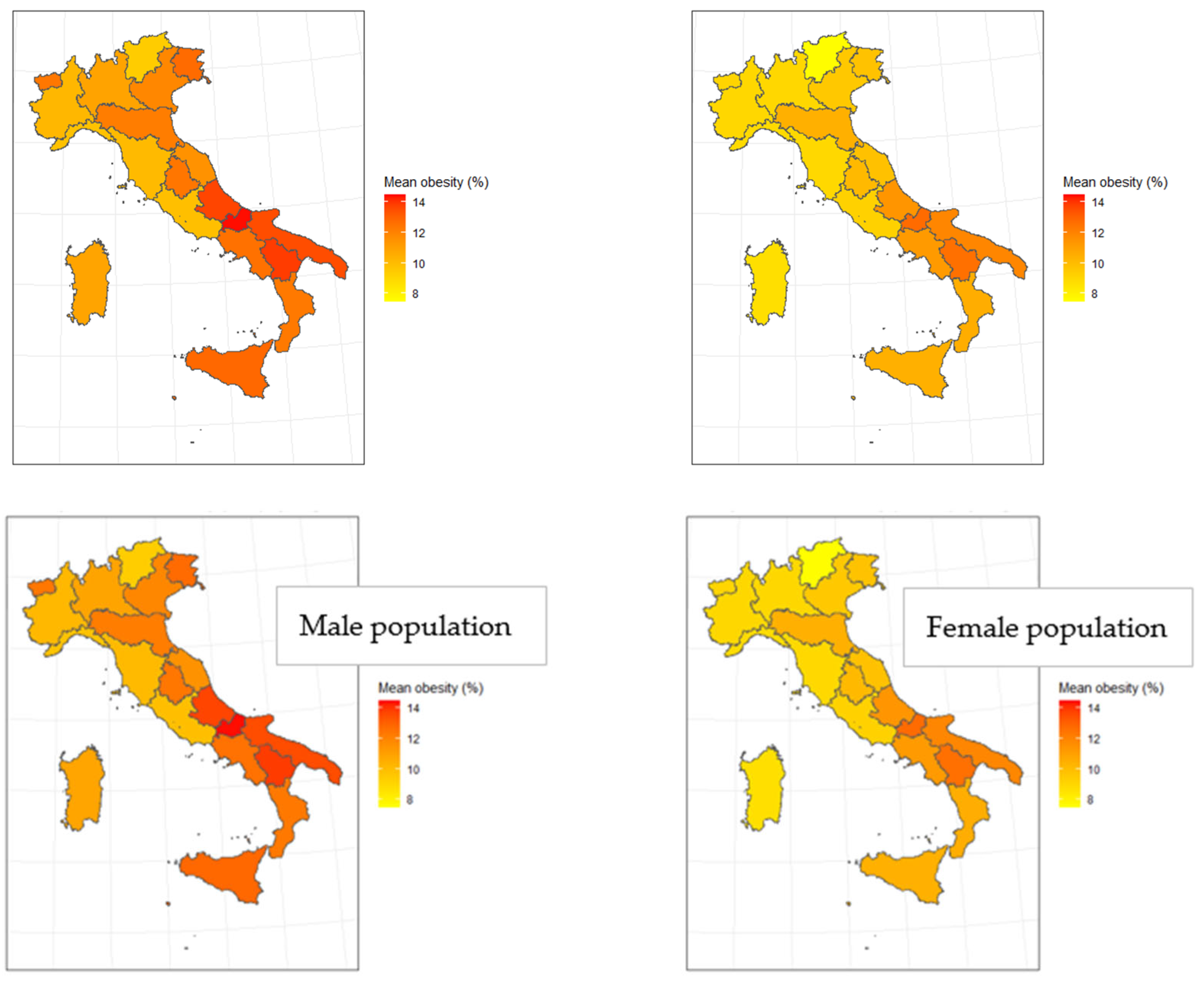
This spatial structure persists also when accounting for gender differences. Figure 2 presents two maps depicting the average obesity, but with a distinction between genders.

The two maps shown in Figure 2 provide further evidence of potential spatial dependence for both genders. Notably, when examining gender differences, the distinction appears to lie more in the magnitude of obesity rates than in the spatial patterns themselves. Over the period considered, males consistently exhibit higher obesity rates than females, on average. However, all genders display similar spatial trends, with the southern regions showing higher obesity rates compared to other areas (please refer also to the following Section 3.2).

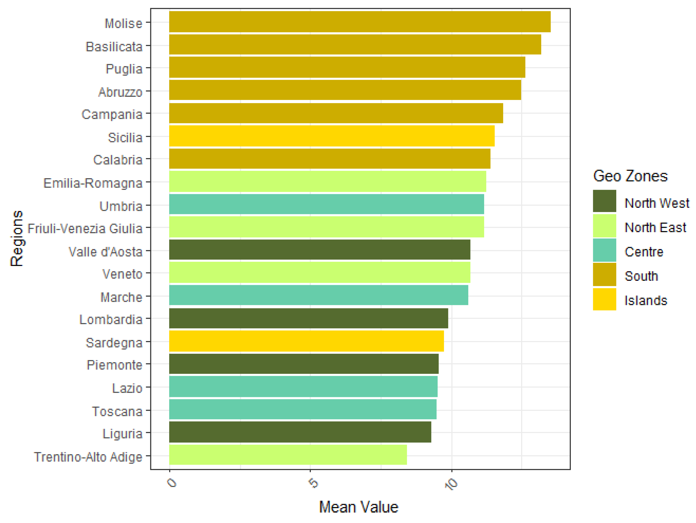
Figure 3 highlights a similar pattern: in this barplot, regions are ordered from the one with the highest average obesity rate (Molise), to the one with the lowest one (Trentino-Alto Adige). They are then categorized into the geographical zones—defined in Table 1—and referred to as ”Geo Zones” in the figure. This visualization highlights the geographical structure of obesity rates, showing that the southern regions consistently have higher values, while other areas are more similar and present lower rates.

By grouping regions into broader geographical zones rather than focusing on them individually, the distribution of average obesity rates is more effectively represented in the box plot shown in Figure 4. This allows for a clearer visualization of their areal tendency. Particularly, the figure depicts the distribution of average obesity rates for all genders and for each geographic zone. The box plot confirms that most zones have relatively similar obesity ranges, with southern area standing out as an exception and presenting a significantly higher prevalence of obesity. Notably, two clear outliers are observed in the Islands region, corresponding to the average obesity values for Sicily in 2021 and 2022, which are particularly high compared to the rest of the country.

Testing the significance of differences in obesity prevalence for different geographical areas, the South of Italy shows significantly higher rates compared to all other zones, with the largest differences observed when compared to the North West and Centre (

Table 2. Obesity prevalence rates comparison between geographical areas (Welch t-test, p-values and confidence interval).

Comparison	Difference	t-Statistic	p-Value	CI Low	CI High
South vs. North East	2.12	8.36	<0.0001	1.61	2.62
South vs. Centre	2.31	10.7	<0.0001	1.89	2.74
South vs. North West	2.65	12.1	<0.0001	2.21	3.08
South vs. Islands	1.85	5.58	<0.0001	1.18	2.52
North East vs. Centre	0.199	0.799	0.426	−0.295	0.694
North East vs. North West	0.531	2.12	0.0364	0.0342	1.03
North East vs. Islands	−0.262	−0.741	0.462	−0.973	0.449
Centre vs. North West	0.332	1.56	0.123	−0.0914	0.755
Centre vs. Islands	−0.461	−1.40	0.169	−1.13	0.204
North West vs. Islands	−0.793	−2.41	0.021	−1.46	−0.126

). Other comparisons are mostly not statistically significant, suggesting more similar obesity patterns across the northern and central regions of Italy.

3.2. Gender Differences in Obesity Prevalence

To assess whether obesity rates differ significantly between males and females, we performed two-sided Welch’s t-tests across various dimensions, including geographical zones (NUTS 2 classification), years, and administrative regions (

Table 3. Obesity prevalence rates comparison between male and female population in Italian regions (Welch t-test, p-values and confidence interval).

Region	Difference Between Male and Female Rates	t-Statistic	p-Value	CI Low	CI High
Abruzzo	2.26	3.80	<0.0001	1.03	3.50
Basilicata	1.26	1.88	0.0735	−0.13	2.65
Calabria	1.78	3.50	0.00186	0.73	2.83
Campania	1.34	2.22	0.0365	0.09	2.59
Emilia-Romagna	1.76	3.67	0.00123	0.77	2.75
Friuli-Venezia Giulia	2.96	6.59	<0.0001	2.03	3.88
Lazio	0.69	1.68	0.106	−0.16	1.53
Liguria	0.97	1.76	0.0915	−0.17	2.10
Lombardia	1.90	6.53	<0.0001	1.30	2.50
Marche	1.70	3.17	0.00429	0.59	2.81
Molise	1.68	2.62	0.0150	0.36	3.00
Piemonte	1.21	3.29	0.00367	0.44	1.98
Puglia	1.59	5.26	<0.0001	0.97	2.22
Sardegna	2.18	5.49	<0.0001	1.36	3.00
Sicilia	2.35	3.63	0.00162	1.00	3.70
Toscana	1.13	2.72	0.0135	0.26	2.00
Trentino-Alto Adige	1.88	5.41	<0.0001	1.16	2.60
Umbria	2.27	6.63	<0.0001	1.56	2.98
Valle d’Aosta	3.26	5.54	<0.0001	2.04	4.48
Veneto	2.31	5.34	<0.0001	1.42	3.21

). Welch’s t-test is robust to unequal variances, making it particularly suitable when comparing subpopulations with potentially heterogeneous variance structures.

Gender differences are significant in every region: the male population shows consistently higher prevalence of obesity than the female population (more than two percentage points), with the exception of the “Lazio” region, where the share of male population with obesity is one percentage point higher than among women.

3.3. Spatiotemporal Analysis

In the visualizations considered so far, the temporal dimension has been aggregated, resulting in the omission of any potential temporal dynamics in conjunction with the spatial ones. In order to consider also the temporal dimension, further visualizations follow. As a starting point, by averaging all the regional values for each geographic area, a time series of each zone is reported in Figure 5.

The time series analysis reveals a clear upward trend in regional obesity rates, averaged by geographical zone, over the period from 2010 to 2022. Notably, the data illustrate evident differences in the southern regions of Italy with respect to the other—more similar—areas, exhibiting consistently higher obesity rates. Despite these differences in the magnitude of the values, the temporal pattern of obesity rates appears similar across all geographical areas. A common trend emerges, since the obesity rate for every area increases from 2010 (with the exception of the central area of Italy), peaks in 2021, and declines again in 2022.

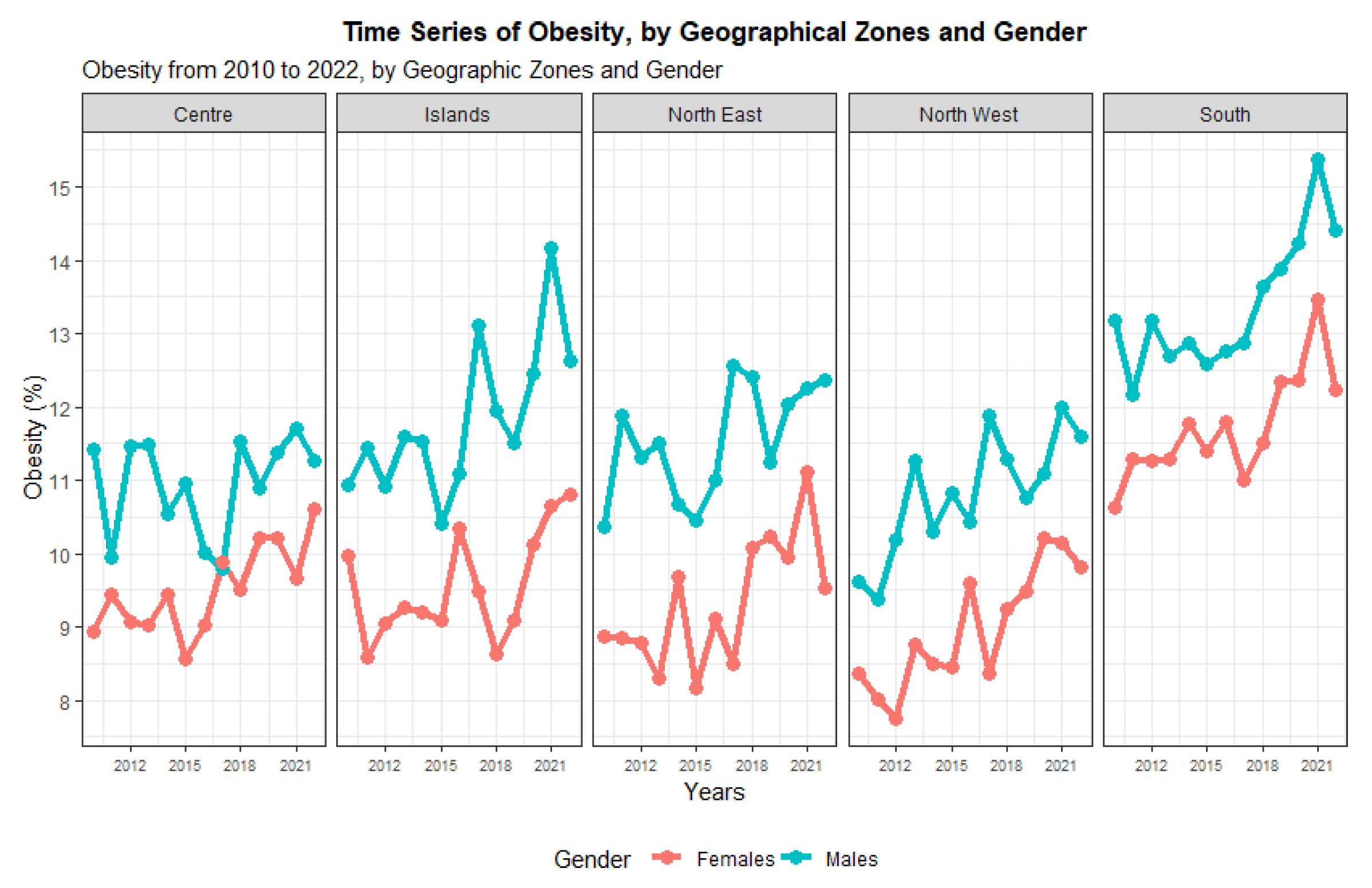
The analysis of trends by sex highlights gender differences (Figure 6): while the temporal trend appears consistent for both genders, without any notable difference, male obesity rates show to be consistently higher than female ones.

Gender differences in obesity prevalence rates are consistent over time: obesity rates are significantly higher for men than for women (

Table 4. Obesity prevalence rates comparison between male and female population, years 2010–2022 (Welch t-test, p-values and confidence interval).

Year	Difference Between Male and Female Rates	t-Statistic	p-Value	Confidence Interval Low	Confidence Interval High
2010	1.91	3.81	0.00054	0.89	2.93
2011	1.53	2.48	0.0175	0.28	2.77
2012	2.23	3.74	0.00061	1.02	3.44
2013	2.29	4.60	<0.0001	1.28	3.30
2014	1.33	2.34	0.0251	0.18	2.49
2015	1.90	3.88	0.00043	0.91	2.89
2016	1.10	2.06	0.0464	0.02	2.19
2017	2.43	4.24	0.00014	1.27	3.58
2018	2.25	4.07	0.00023	1.13	3.37
2019	1.29	2.08	0.0442	0.04	2.55
2020	1.62	2.95	0.00564	0.51	2.73
2021	1.93	2.89	0.00633	0.58	3.28
2022	1.90	3.77	0.00055	0.88	2.91

). As well as the prevalence of obesity among men and women showing no signs of decline, in the same way, the gender gap does not present a significant decrease. Even if the difference between male and female obesity rates reached a maximum in 2017, with a value of 2.43 percentage points, the gap is still high in 2022.

While these time series visualizations effectively capture the overall temporal structure across macro-areas, they miss the interesting regional-level details, as they represent only the average obesity rate for each geographical zone. To address this limitation, we employ a time series box plot that allows us to visualize the temporal behavior while maintaining a geographical focus and assesses the regional variability among geographic areas for each year. Figure 7 presents this time series box plot, which displays the distribution of obesity rates across regions within each macro-area annually.

With the exception of the central area of Italy, where there seems to be some stability over time, a significant increase in the prevalence of obesity occurs in Italy. To note that the variability of the distribution captured by the boxes (hence the difference among regions for each year, by geographic zone) increases for the Islands over time, while it remains quite stable for the other zones, suggests that the regions of Sicily and Sardinia over time differ more. Another interesting observation is the consistent presence of only one low outlier in the North East zone, Trentino-Alto Adige, where obesity rates are consistently lower than the other north-eastern regions.

To conclude the spatiotemporal visualization, it is insightful to examine maps displaying crude obesity rates for specific years, allowing for the observation of potential changes over time, spatial structures and gender differences. Figure 8 presents these maps for eight selected years between 2010 and 2022, with data captured at two-year intervals. Given the trends already observed above (Figure 5), the selection of these particular years does not affect the results of the analysis.

These visualizations confirm findings discussed above in the study. From a spatial perspective, a structure in obesity rates emerges, with neighboring regions exhibiting similar values, indicating a degree of spatial correlation. From a temporal perspective, there is a clear upward trend in obesity rates over the period considered, with males consistently showing higher rates than females. This trend is reflected in the progressive shift in color gradients on the maps between 2010 and 2022, highlighting the increasing prevalence of obesity.

Firstly, the female population shows consistently lower obesity rates than the male one. Furthermore, observing the darker coloring of the maps, it is possible to see it expanding during the time period in analysis, starting from the southern regions, extending to the eastern areas of Italy, and finally involving also the northern regions of Italy, with the only exception of Trentino-Alto Adige. The spreading of the issue, quite interestingly, concerns both the female and male sub-populations, but at different levels of severity.

3.4. Spatial Autocorrelation and Smoothing Analysis

The Moran’s Index provides an indication of the strength of the spatial association, that is to say, the similarity between neighboring regions.

Table 5. Moran’s I values for male and female obesity rates across Italian regions (excluding Sardinia) over the period 2010–2022.

Year	Males				Females
	Moran’s I	p-Value	CI Low	CI Up	Moran’s I	p-Value	CI Low	CI Up
2010	0.501	0.001	−0.341	0.277	0.217	0.045	−0.340	0.257
2011	0.062	0.221	−0.349	0.290	0.283	0.021	−0.329	0.262
2012	0.137	0.103	−0.320	0.262	0.238	0.038	−0.353	0.274
2013	−0.043	0.459	−0.333	0.268	0.206	0.063	−0.313	0.285
2014	0.132	0.127	−0.324	0.282	0.200	0.073	−0.334	0.305
2015	0.206	0.063	−0.333	0.296	0.561	<0.001	−0.325	0.258
2016	0.024	0.329	−0.329	0.285	0.359	0.009	−0.331	0.285
2017	0.099	0.185	−0.307	0.303	0.224	0.044	−0.335	0.284
2018	0.078	0.201	−0.329	0.274	0.115	0.142	−0.323	0.271
2019	0.143	0.122	−0.327	0.286	0.158	0.084	−0.344	0.266
2020	0.075	0.186	−0.326	0.245	0.478	<0.001	−0.324	0.251
2021	0.433	0.003	−0.336	0.282	0.403	0.002	−0.340	0.281
2022	0.365	0.006	−0.316	0.285	0.451	0.002	−0.353	0.280

below presents Moran’s I values for male and female obesity rates across Italian regions (excluding Sardinia) over the period 2010–2022. Trends of Moran’s Index suggest spatial association among regions (values higher than zero) for both genders, consistently over time.

The observed values of Moran’s I vary over time, but several patterns emerge. In general, the index is quite volatile among years, but it shows almost always some spatial covariance among regions. Interestingly, the spatial dependence shows up to be (with the exceptions of the years 2010 and 2021) higher for females than for males: spatial clustering of obesity rates is more consistently pronounced in the female population across the study period. For males, the pattern is more sporadic, with isolated years of significance (notably 2010, 2021, and 2022), while for female population significant years—particularly 2015, 2016, 2020, 2021, and 2022—show Moran’s I values well above the null distribution, suggesting a stronger spatial concentration of obesity prevalence. These patterns may reflect differential regional factors affecting male and female populations. Overall, spatial clustering appears more stable and pronounced in the female population, which could point to gender-specific regional determinants (see Section 3.5), and it could also potentially indicate different health policy impacts in the future.

The choropleth maps in Figure 9 display the smoothed obesity rate values for each region, focusing on every two years between 2010 and 2020, and 2021 and 2022, allowing for a direct comparison to maps in Figure 8. If Moran’s I is significantly positive, the smoothed maps reveal consistent spatial gradients—as indeed seen in this analysis, where obesity rates gradually increase from northern to southern regions. As described in Section 2.4, smoothed values take into account spatial similarities, therefore allowing a more meaningful visualization of potential spatial dependence.

By comparing the smoothed maps in Figure 9 with those displaying crude obesity rates in Figure 8, it becomes clear that the smoothing technique helps in visualizing spatial and temporal structures in a more ”uniform” manner. For all the years examined, a gradient in smoothed values is evident, with obesity rates generally increasing from north to south, across both genders. Additionally, the temporal trend of rising obesity rates over the years is visible in the smoothed maps.

The spatial and temporal structures revealed by this smoothing technique provide valuable insights, highlighting potential patterns of interest and confirming strong territorial disparities.

3.5. Extension: Spatiotemporal Analysis of Islands

In spatial statistical analysis, islands or spatial units with no immediate neighbors pose unique challenges, particularly when constructing spatial weights matrices. Contiguity-based methods, like the one employed in this study, may leave islands with no defined neighbors, leading to missing values or computational issues in models that rely on spatial dependence [26]. Our analysis considers the concept of adjacency as neighborhood, using a weights matrix W where entries w_ij = 1 if i∼j and w_ij = 0 elsewhere (including w_ii), following the main literature on spatial statistics with areal data, where “1” indicates regions with a shared border, and 0 for regions with no touching border, as extensively described in Section 2.2 [16,17]. Therefore, in the case of Italian regions, one could think of the islands of Sicily and Sardinia in different cases:

1.

Treating the two islands as two separate entities, with no neighbors.

2.

Treating Sicily as a neighbor of Calabria, because of the very near distance, but with Sardinia separated from all.

3.

Treating Sicily and Sardinia as neighbors (with Sicily also being neighbor of Calabria).

The calculated Moran’s I values, apart from being quite variable through time, show also some differences based on the three specified neighborhood criteria. Figure 10 presents three plots illustrating the Moran’s I statistics across the time points from 2010 to 2022, comparing the three neighborhood classifications for Sicily and Sardinia. In these plots, the Moran’s I values are displayed on the y-axis, while the years are plotted along the x-axis. For better readability, each plot includes five horizontal reference lines: a solid red line at 0, red dashed lines at ±0.05, and orange dashed lines at ±0.1. There is no particular choice in those values, which serve just as a reference in the plot for little-to-no spatial correlation.

In the first plot (“With only Sicily”), the weights matrix W treats Sicily as a neighbor of Calabria, while Sardinia is considered an isolated region. In the second plot (“With Sicily and Sardinia”), W assigns both Calabria and Sardinia as neighbors of Sicily, with Sardinia also considered a neighbor of Sicily. In the final plot (“Without Sicily and Sardinia”), Sicily and Sardinia are treated as completely separate entities, with no neighbors. These distinctions provide a clearer visualization of the temporal evolution of spatial correlation in obesity rates across the different neighborhood classifications.

We can conclude that considering these regions as isolated identities does not significantly affect the Moran’s I coefficient values, because of the ambiguity surrounding their treatment in the spatial analysis: considering Sicily as a neighbor of Calabria and Sardinia as an isolated region, including Sardinia as a neighbor of Sicily, or excluding both regions entirely seems not to affect significantly the analysis. Finally, it is worth mentioning that excluding the two regions from the smoothing procedure is also consistent with the standard queen contiguity method, as implemented in the R spdep package, that in fact automatically assigns a weight of zero to islands [27].

3.6. Spatial Analysis of Determinants of Regional Prevalence Rates of Obesity

To reduce obesity prevalence and its regional disparities, it is important to make intervention and prevention efforts, taking into account the socioeconomic and physical environmental characteristics of the region as well as health behaviors. In order to optimize the targeting of public health resources, in addition to the spatial variation of obesity prevalence, it is useful to analyze its associations with socio-economic and behavioral factors (e.g., food environment, physical activity). In this way, it is possible to provide some hints of the reasons behind differences in the prevalence of obesity between adjacent regions. Sociodemographic characteristics of the population including household income and unemployment rate have been identified as regional determinants of obesity [13,28,29,30]. In addition, healthy behaviors such walking practice, participation in social activity, vegetables daily intake were associated with different levels of regional obesity [30].

Figure 11 shows that regions with higher unemployment and higher shares of the population which does not practice sports (inactive population) are also those regions where obesity is more frequent among adults. Furthermore, in regions where the share of population having their daily intake of vegetables is lower, the prevalence of obesity is higher. This result is consistent with studies underlying the “crisis” of the Mediterranean diet: despite the well-documented advantages of this diet, many countries in the Mediterranean area, including Italy, are experiencing a progressive shift away from this dietary model, determining high rates of obesity [31].

In continuity with previous research, regions with lower levels of education also present higher prevalence ratees of obesity [13,29].

This analysis is only a starting point in the study of the determinants of regional inequalities in obesity and a more thorough study is needed.

4. Discussion

The overall obesity rate increases over the 13 years considered and the spreading trends of obesity in Italy over time derived from this study are coherent with previous studies [31]. On this basis, we used spatial autocorrelation analysis to study the spatial and temporal evolutionary trends of obesity rates in Italian regions, exploring the spatial distribution characteristics of obesity rates at a deeper level.

The results of the spatial autocorrelation analysis in this study showed that, in general, obesity rates between 2010 and 2022 had a strong positive spatial correlation. Although the spatial clustering of obesity does not present a significant trend, obesity shows positive spatial correlations in the whole period.

This study highlights how in 2015 and in the latest years between 2020 and 2022, the spatial patterns of obesity rates are particularly high. Obesity trends presented specific challenges during the COVID-19 lockdowns, due to abrupt lifestyle changes, limited access to healthcare and physical activity, and shifts in dietary patterns. The lockdowns intensified sedentary behavior and emotional eating, complicating efforts to distinguish temporary weight gain from long-term obesity trends [32,33]. This study, thus, extends to Italy results of previous studies related to the increasing of obesity prevalence rates during the COVID-19 lockdown.

Moreover, the spatial treatment of island regions like Sicily and Sardinia posed analytical challenges, due to their geographic isolation and lack of contiguous borders with other regions. This study poses an important contribution to the analysis of islands, demonstrating that results of Moran’s Index do not change significantly according to the different possible ways of considering borders: Sicily as a neighbor of Sardinia, Sicily and Sardinia as isolated areas (as foreseen by Bivand’s methods), or considering Sicily a neighbor of Calabria, because of their minimal distance and Sardinia as an isolated area. The demonstration that these three methods provide similar results can be useful for official statistics and provides indication on possible alternative classifications.

This study presents a valuable spatiotemporal analysis of adult obesity in Italy, yet it is important to acknowledge some limitations that may influence the interpretation and generalizability of the findings. First, obesity was measured using Body Mass Index (BMI), following the WHO threshold of BMI ≥ 30. Although BMI is a widely used proxy in population health studies, it has well-known limitations, particularly its inability to differentiate between fat and lean mass or to account for fat distribution and metabolic health. This can lead to misclassification, especially in older adults or those with higher muscle mass [13,15].

Second, the analysis based on aggregated regional data (NUTS 2 level) would benefit from an extension at the individual level [9]. The findings of this study should be interpreted with caution when informing individual-level health policies or interventions. Furthermore, although the study explores associations between regional obesity prevalence and socioeconomic indicators such as unemployment, inactivity, education, and diet, these analyses remain preliminary and largely descriptive. A more rigorous analytical approach—such as multilevel modeling—would be necessary to disentangle the complex interplay between individual-level behaviors and contextual determinants [9,34].

Furthermore, the analysis of socio-economic and behavioral determinants of obesity is exploratory and descriptive: the associations shown (e.g., unemployment, inactivity, low education, low vegetable intake) could be formally modeled and a wider range of determinants can be investigated, in order to provide further information to overcome obesity.

Lastly, although gender differences were addressed, the study did not explore age-stratified trends, potentially overlooking generational-specific dynamics.

Future research should build upon this work by employing individual-level longitudinal data, integrating environmental variables (e.g., food deserts, green space), and applying spatially explicit multilevel models.

5. Conclusions

This paper provides a comprehensive analysis of the spatial and temporal dynamics of obesity rates across Italian regions from 2010 to 2022. By integrating data visualization techniques with spatial analysis, the study uncovers key insights into regional disparities and temporal trends in obesity, emphasizing the influence of geographic, temporal, and gender-related factors.

The findings indicate pronounced geographic disparities in obesity rates across Italy, with southern regions consistently exhibiting a higher prevalence compared to northern areas. This spatial variation aligns with and extends previous research, suggesting that differences in physical activity, dietary patterns, and socioeconomic conditions contribute to this divide. Notably, the analysis confirms a significant spatial dependence in average obesity rates, underscoring the importance of regional context in understanding public obesity trends. In addition, the study reveals gender-specific spatial patterns, with obesity rates persistently higher among males across the country.

Findings from this research contribute to the broader literature on spatial epidemiology and obesity determinants. By incorporating geographic information into obesity analysis, this study highlights the importance of targeted regional policies and interventions. The integration of spatial and temporal modelling techniques provides a robust framework for understanding obesity dynamics, informing future research and public health strategies.

This study indicates that while overall obesity rates in Italy have shown periods of stabilization or modest increases, significant regional and gender disparities persist. Particularly concerning are higher obesity rates in southern regions and among male populations. The peculiar characteristics of Italian regions and the persistent spatial association of obesity prevalence underline that policies aiming to tackle excess adiposity and obesity should address both people and places.

Although these results need confirmation through further systematic and periodic monitoring, they have major public health implications and justify the strengthening of initiatives undertaken for the reduction in obesity in Italy by the National prevention plan 2020-25 [35], underlining that attention should be paid to gender differences, thereby reducing disparity, and of the recent Guidelines for the prevention and management of overweight and obesity [36], drawn at the regional level and aimed at promoting healthy diets and physical activity.

Continued public health efforts are essential to address these disparities and promote healthier lifestyles across all demographics.