Predicting Hydrogen Production from Steam Methane Reforming Powered by Induction Heating: An Application of a Hybrid Bayesian Neural Network

Abstract

Steam methane reforming (SMR) powered by induction heating offers a promising route for low CO₂-emission hydrogen production, but predictive modelling remains challenging because the available experimental data are limited and heterogeneous. This study proposes a hybrid Bayesian neural network (H-BNN) to predict the mass of hydrogen (MoH) from literature-derived SMR data using operating variables including temperature, flow rate, power input, time-on-stream, and interval duration. Feedforward neural network (FNN) and classical Bayesian neural network (BNN) models were also developed as benchmarks, and all three architectures were evaluated with ReLU, Tanh, and GELU activation functions. To address data scarcity, only the training split was augmented at scales of $k=2$, 5, and 10, while the validation and test sets were kept unchanged. The H-BNN combines deterministic feature extraction with Bayesian uncertainty-aware prediction, enabling a balance between accuracy and uncertainty representation. Across the validation-selected models, test performance reached R² ∼ 0.9894 to 0.9969, with mean absolute errors of 0.0126 g to 0.0217 g. The strongest advantage appeared at k = 2, where the H-BNN outperformed the benchmark models. Overall, the proposed H-BNN is a promising framework for hydrogen prediction under data-scarce conditions, although its predictive intervals remain informative rather than fully calibrated.

1. Introduction

Steam Methane Reforming (SMR) is a pivotal industrial process for hydrogen generation that primarily converts methane and steam into hydrogen and carbon monoxide at elevated temperatures [1]. This endothermic reaction normally occurs over a nickel-based catalyst in tubular reactors housed in gas-fired furnaces [2]. The process typically works at 700–1000 °C with pressures ranging from 3 to 25 bar to convert natural gas feedstock into syngas [1,3]. The created carbon monoxide can then undergo a water-gas shift reaction with more steam, yielding more hydrogen and carbon dioxide in a somewhat exothermic process [4].

As shown in Figure 1, the SMR is a well-established pathway for large-scale hydrogen production; however, it requires substantial energy input owing to the highly endothermic primary reforming step (See Figure 2), which is usually powered by non-renewable fuels [5,6]. The conventional steam methane reforming process mainly comprises Steam Methane Reforming (SMR) and the Water Gas Shift Reaction (WGSR):

Steam Methane Reforming (SMR):

$$C{H}_4+H_{2}O\rightleftharpoons CO+3H_2\Delta H=+206\mathrm{kJ}/\mathrm{mol}$$

Water Gas Shift Reaction (WGSR):

$$CO+H_{2}O\rightleftharpoons C{O}_2+H_2\Delta H=-40\mathrm{kJ}/\mathrm{mol}$$

Alternatively,

Direct Steam Reforming (DSR):

$$C{H}_4+2H_{2}O\rightleftharpoons C{O}_2+4H_2\Delta H=+165\mathrm{kJ}/\mathrm{mol}$$

Furthermore, according to Le Châtelier’s principle, SMR requires a lower pressure despite being a highly endothermic reaction. Typically, in large-scale scenarios, the outlet temperature ranges from 850 °C to 950 °C to achieve optimum methane conversion [1,2,5]. Industrial SMR processes typically operate at higher pressures to boost throughput and minimize equipment size, thus necessitating even higher temperatures to sustain a favorable equilibrium for hydrogen production [1].

Despite widespread deployment, steam methane reforming (SMR) operates at elevated temperatures and pressures, resulting in a significant carbon footprint. From a global perspective, SMR facilities account for nearly 3% of all CO₂ emissions [2,5]. Consequently, this substantial environmental impact underscores the urgent need to develop sustainable hydrogen production methods and integrate carbon capture technologies into existing SMR plants.

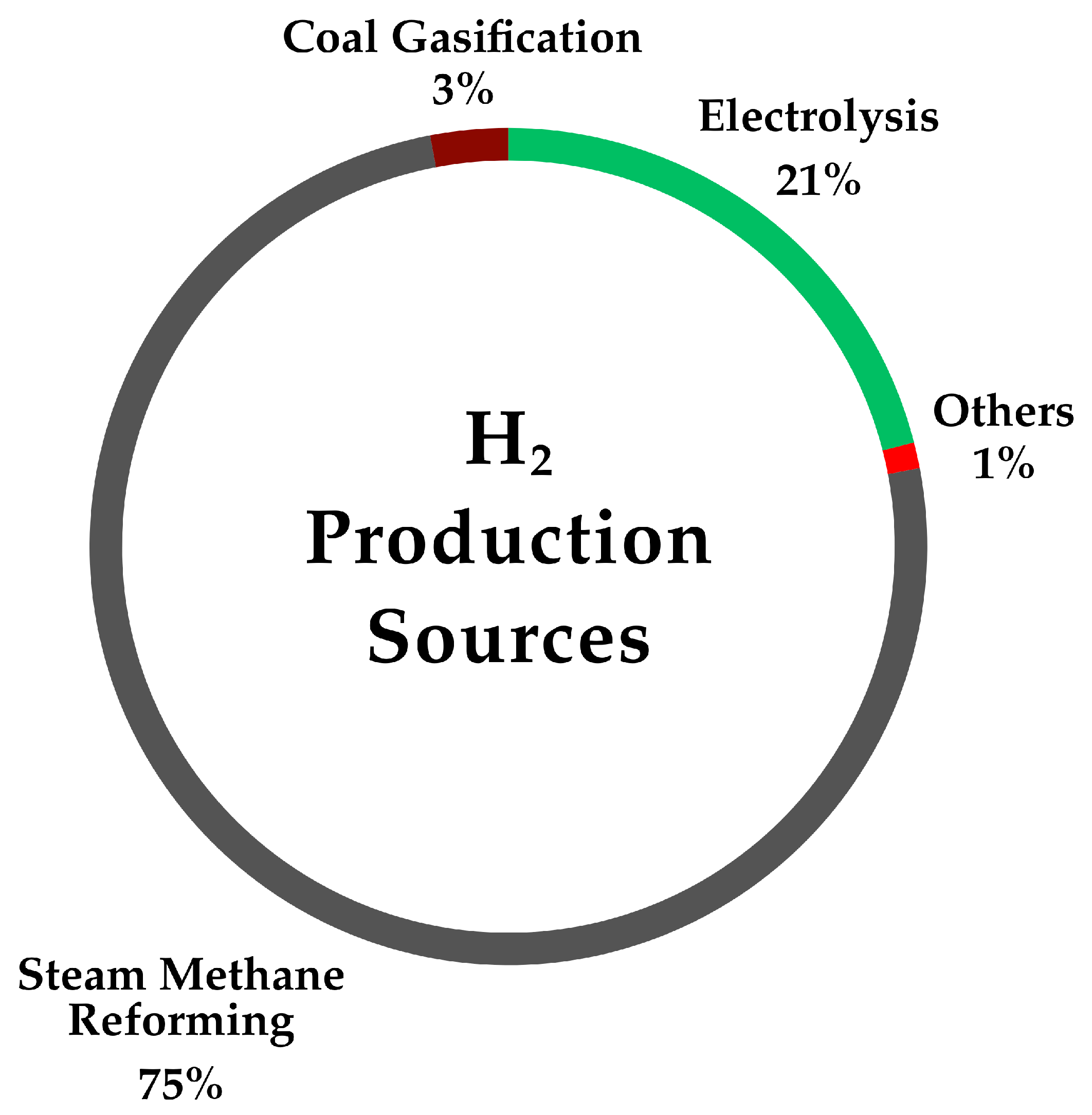
Figure 1. The donut chart above reveals the current global most adopted Hydrogen gas (H₂) production pathways. The Steam Methane Reforming (SMR) is about ∼75% as shown. Thus, this reveals both the Technological and Commercial Readiness Level (TRL & CRL) of the SMR production for the production of Hydrogen gas (H₂). The donut chart is based on data reported in [7,8,9].

Figure 1. The donut chart above reveals the current global most adopted Hydrogen gas (H₂) production pathways. The Steam Methane Reforming (SMR) is about ∼75% as shown. Thus, this reveals both the Technological and Commercial Readiness Level (TRL & CRL) of the SMR production for the production of Hydrogen gas (H₂). The donut chart is based on data reported in [7,8,9].

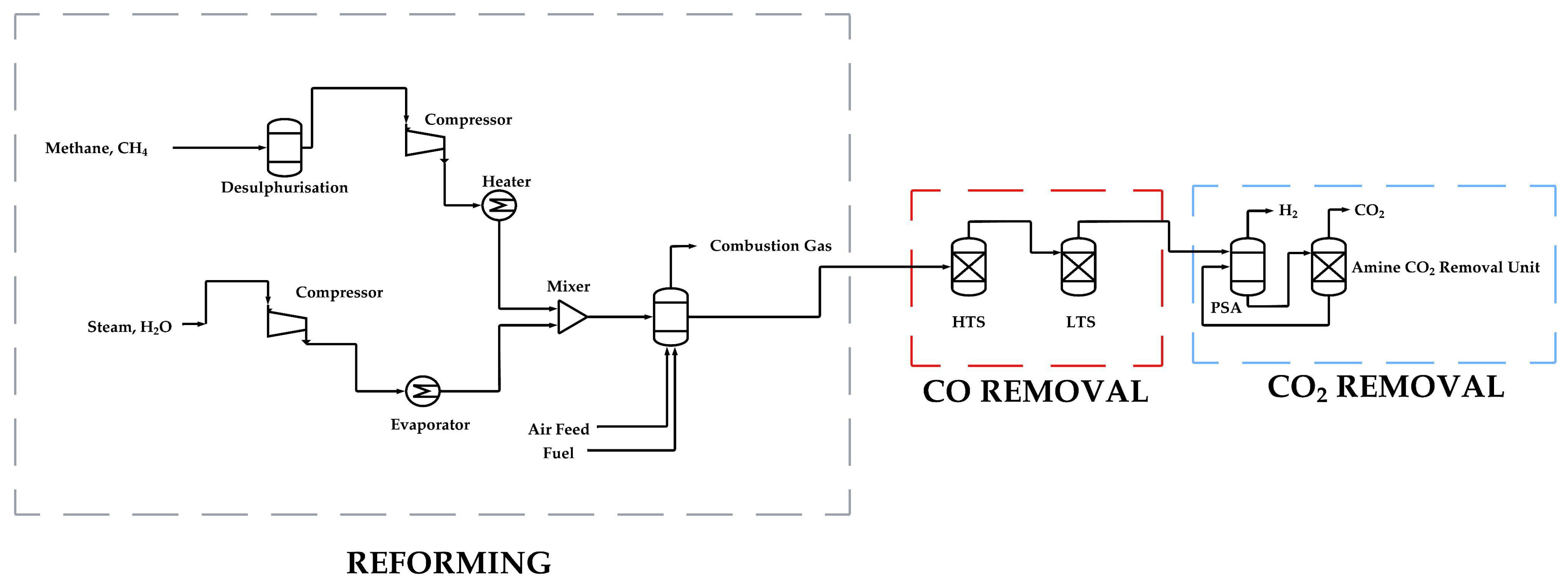
Figure 2. The schematic diagram above presents the conventional Process Flow Diagram (PFD) for conventional Steam Methane Reforming (SMR). The SMR process encompasses multiple stages for the production of blue hydrogen (H₂), facilitated by the carbon (IV) oxide (CO₂) capture unit. Additionally, as depicted in the CO removal process indicated by the red dotted line, the SMR incorporates two water-gas shift (WGS) reactors: a high-temperature shift (HTS) and a low-temperature shift (LTS). While CO₂ is absorbed by the Amine CO₂ removal unit, hydrogen (H₂) is generated via the Pressure Swing Adsorption Unit. The blue dotted boundary line delineates the supplementary carbon-capturing units necessary to achieve net-zero emissions targets. It worth noting that this conceptual schematic process flow diagram was based on [10,11].

Figure 2. The schematic diagram above presents the conventional Process Flow Diagram (PFD) for conventional Steam Methane Reforming (SMR). The SMR process encompasses multiple stages for the production of blue hydrogen (H₂), facilitated by the carbon (IV) oxide (CO₂) capture unit. Additionally, as depicted in the CO removal process indicated by the red dotted line, the SMR incorporates two water-gas shift (WGS) reactors: a high-temperature shift (HTS) and a low-temperature shift (LTS). While CO₂ is absorbed by the Amine CO₂ removal unit, hydrogen (H₂) is generated via the Pressure Swing Adsorption Unit. The blue dotted boundary line delineates the supplementary carbon-capturing units necessary to achieve net-zero emissions targets. It worth noting that this conceptual schematic process flow diagram was based on [10,11].

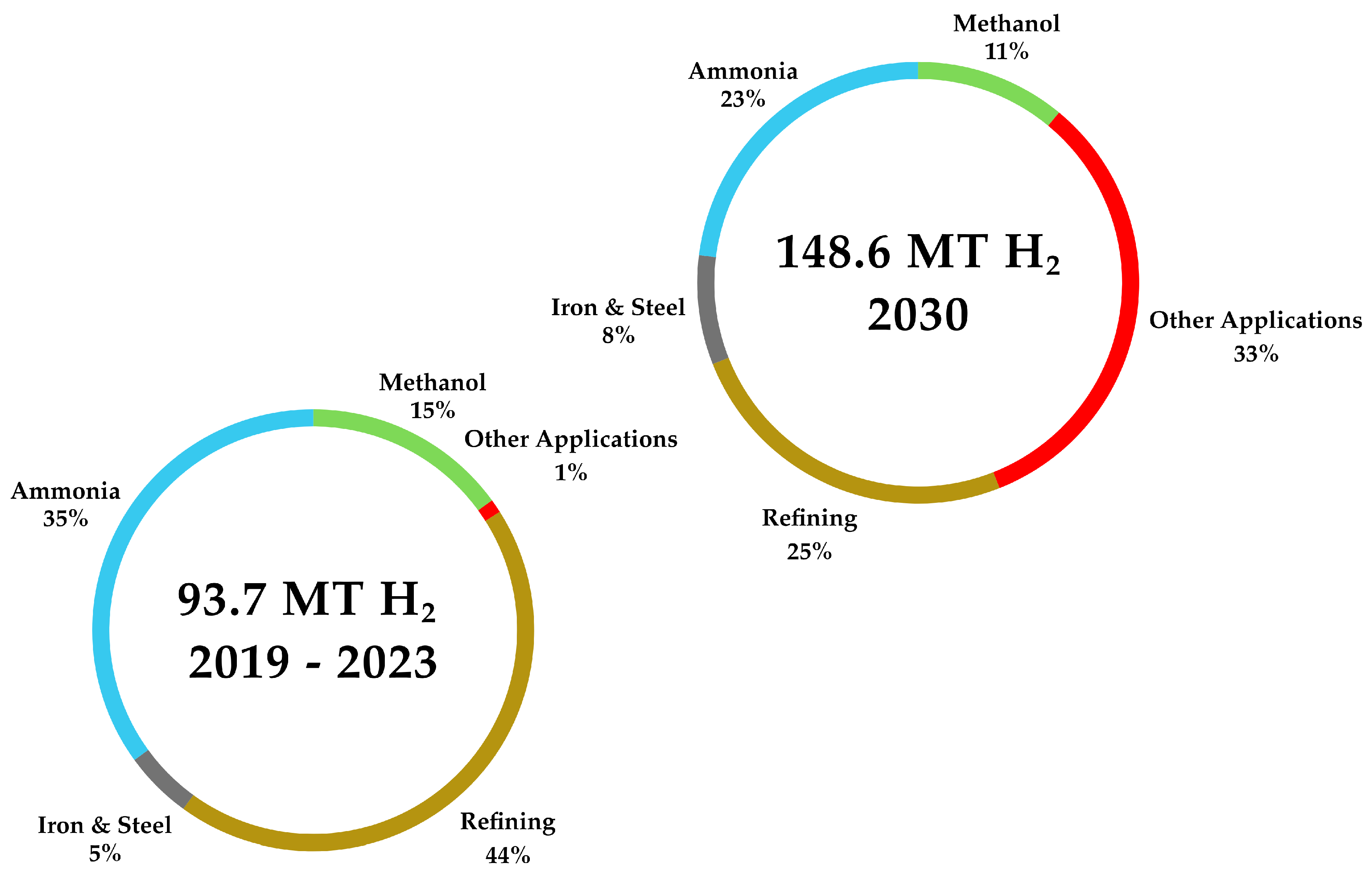
Hydrogen is increasingly recognized as the cornerstone of global energy transition, offering a carbon-free energy carrier that can decarbonize sectors that are difficult to abate, such as heavy industry, chemicals, and long-haul transportation [12,13]. The donut chart in Figure 3 shows global hydrogen consumption in megatonnes (Mt) per year in various sectors. The donut chart on the left in Figure 3 shows the hydrogen consumption for methanol, refining, iron and steel, ammonia, and other applications, totalling approximately 93.7 Mt per H₂ over the period of 2019 to 2023. Similarly, the donut chart on the right side reveals the projection of the International Energy Agency’s Net Zero Emissions (IEA-NZE) for 2030, totaling an estimated 148.6 Mt per H₂.

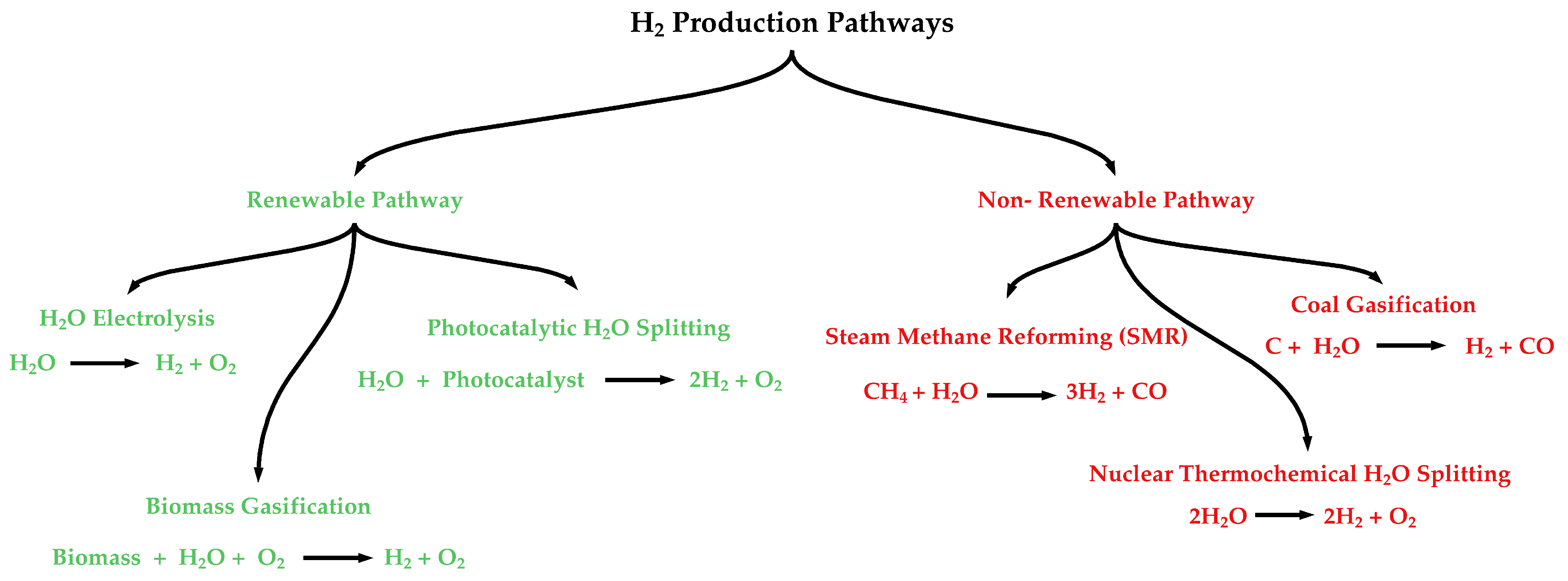
Despite the promise of hydrogen as a clean energy carrier, its sustainability is predicated on its production method. As depicted in Figure 4, hydrogen can be produced from renewable (green pathways) or non-renewable sources (grey, blue, or black pathways). However, the Steam Methane Reforming process is primarily associated with non-renewable sources, which results in the production of grey hydrogen. Furthermore, when SMR is combined with carbon capture and storage (CCS), the resulting hydrogen is typically referred to as blue hydrogen. This classification highlights the dual challenge of SMR despite its technological maturity, it remains carbon-intensive unless emissions are mitigated effectively.

However, the sustainability of hydrogen production remains a challenge. Currently, most hydrogen is produced by steam methane reforming (SMR), a process that emits significant amounts of CO₂ unless paired with costly carbon capture and storage (CCS) systems. This dependence on fossil-based hydrogen has prompted the search for alternative production pathways that combine economic viability with deep decarbonization potential [16,17,18].

A process flow diagram (PFD) illustrates a schematic for Steam Methane Reforming powered by Induction Heating (IH), leading to the production of hydrogen (H₂) and capture of carbon (IV) oxide (CO₂), as depicted in Figure 2. The investigation or training of the proposed hybrid Bayesian neural network was based on various input data, such as Methane Conversion (%), Time on Stream (TOS) on the catalytic surface, Power Input (W), Temperature (°C), Magnetic Flux, and other significant variables that influence steam methane reforming through induced heating.

Recently, modern SMR systems have integrated artificial intelligence, machine learning, and data-driven optimization to enhance reactor control, improve predictive accuracy, and reduce emissions. Moreover, hybrid physics-informed models and digital twins can facilitate improved forecasting of hydrogen yield and operational degradation processes, exceeding the capabilities of traditional models [19,20].

The methodology employed in this study is more accurately characterized as a bootstrap-based Gaussian jittering data-augmentation strategy, as opposed to other data augmentation approaches. While this stochastic augmentation does not replace a systematic exploration of the input space, it is applied solely to the training subset thus providing a controlled, transparent, and reproducible means of enriching limited experimental data in a manner consistent with plausible measurement uncertainty.

Within this framework, the Hybrid Bayesian Neural Network (H-BNN) particularly benefits from the augmented data, as the additional perturbed samples facilitate more stable parameter learning while maintaining uncertainty-aware prediction. As a result, the H-BNN framework is not only more reproducible from a modelling perspective but also more practically applicable for reliable hydrogen-production forecasting, as well as further analysis, such as post-processing of derived performance indicators, including hydrogen yield (Y_H2) and specific energy consumption (SEC). Consequently, SMR can bridge established industrial practices and innovations, with its future deployment depends on advancements in carbon capture, methane leakage control, AI-driven optimization, and economic alignment with renewable hydrogen production [20,21,22].

In this study, a hybrid Bayesian Neural Network (H-BNN) framework was developed and deployed to predict hydrogen gas production generated from steam methane reforming via induction heating. The dataset used in the training (70%) of the H-BNN was scarce hence the theme of this study. Furthermore, the training set of the dataset was scaled up to a ten times to optimally train the proposed neural network frameworks. It is worth noting that the test (15%) and validation (15%) sets were left unadulterated to maintain the integrity of the datasets and prediction efficiency of the H-BNN.

1.1. The Hybrid-Bayesian Neural Network (H-BNN)

A Hybrid Bayesian Neural Network (H-BNN) combines the deterministic function-approximation capability of a standard Feedforward Neural Network (FNN) with the uncertainty-quantification capacity of a Bayesian approximation. In the present study, the objective was to preserve the strong predictive performance of a deterministic neural network while simultaneously quantifying predictive uncertainty in the estimation of hydrogen production. Accordingly, the H-BNN was designed as a deterministic FNN backbone regularized through Monte Carlo (MC) dropout, which enables an efficient approximation to Bayesian inference.

The central idea is to retain dropout during both training and inference so that the network can be interpreted as sampling from an approximate posterior distribution over the weights. Following the variational interpretation of dropout established by Gal and Ghahramani (2016), the repeated application of dropout at different layers may be viewed as an approximate variational inference scheme in a deep probabilistic model [23,24]. In this manner, the H-BNN preserves the computational simplicity of a conventional FNN while incorporating a practical mechanism for uncertainty estimation. It is important to acknowledge that this interpretation is approximate and is based on simplifying assumptions. Therefore, in the present study, MC dropout was employed as a computationally efficient method for approximating uncertainty, rather than as an exact representation of Bayesian posterior inference.

1.2. Monte Carlo Dropout and Kullback–Leibler (KL) Divergence

1.2.1. Monte Carlo Dropout

Monte Carlo (MC) dropout is a stochastic regularization and approximate inference technique in which dropout remains active during both training and inference. In this setting, each forward pass samples a different subnetwork of the full model, thereby yielding a stochastic prediction of the form:

$${\widehat{y}}^{\left(t\right)}=f(\mathbf{x};W^{\left(t\right)}),W^{\left(t\right)}\sim q\left(W\right)$$

(1)

where $q\left(W\right)$ denotes the approximate variational distribution induced by dropout. Repeated forward passes for the same input produce a set of stochastic outputs, ${\widehat{y}}^{\left(1\right)}$, ${\widehat{y}}^{\left(2\right)}$, …, ${\widehat{y}}^{\left(T\right)}$, from which the predictive mean and predictive variance can be estimated as

$$\mu ={\displaystyle \frac{1}{T}}{\displaystyle \sum _{t=1}^T}{\widehat{y}}^{\left(t\right)},{\sigma }^2={\displaystyle \frac{1}{T}}{\displaystyle \sum _{t=1}^T}{\left({\widehat{y}}^{\left(t\right)}-\mu \right)}^2$$

(2)

Here, $\mu$ represents the mean prediction across the T stochastic forward passes, whereas ${\sigma }^2$ provides an estimate of predictive uncertainty arising from the approximate posterior over the weights.

1.2.2. KL Divergence in Variational Inference

In Bayesian learning, the true posterior distribution of the weights, p(W $\mid \mathcal{D}$), is generally intractable. Variational inference therefore introduces a tractable approximation $q\left(W\right)$ and seeks to minimize the Kullback-Leibler (KL) divergence between the approximate and true posteriors:

$$\mathrm{KL}\left(q\left(W\right)\parallel p(W\mid \mathcal{D})\right)=\int q\left(W\right)\log \left({\displaystyle \frac{q\left(W\right)}{p(W\mid \mathcal{D})}}\right)dW$$

(3)

Because direct minimization of Equation (3) is not computationally convenient, the optimization is instead formulated through the evidence lower bound (ELBO), given by

$${\mathcal{L}}_{\mathrm{ELBO}}={\mathbb{E}}_{q\left(W\right)}\left[\log p(\mathcal{D}\mid W)\right]-\mathrm{KL}\left(q\left(W\right)\parallel p\left(W\right)\right)$$

(4)

Maximizing L_ELBO is equivalent to minimizing $\mathrm{KL}\left(q\right(W)\parallel p(W\mid \mathcal{D}\left)\right)$. For model training, however, the objective is more conveniently expressed in minimization form as the negative ELBO. In the present H-BNN framework, this variational objective is approximated in practice by a prediction-error term together with a regularization term:

$${\mathcal{L}}_{\mathrm{Hybrid}}\approx \underset{\mathrm{negative} \text{log-likelihood} \mathrm{surrogate}}{\underbrace{{\displaystyle \frac{1}{N}}\sum _{i=1}^N{(y_i-{\widehat{y}}_i)}^2}}+\underset{\mathrm{KL} \mathrm{regularization} \mathrm{surrogate}}{\underbrace{\lambda \sum _l{\parallel W_l\parallel }_2^2}}$$

(5)

where the first term corresponds to a mean-squared-error approximation of the negative log-likelihood under a Gaussian observation assumption, and the second term serves as a tractable surrogate for the KL regularization implied by the variational formulation. Thus, the H-BNN combines accurate deterministic learning with an approximate Bayesian treatment of weight uncertainty.

As shown in the algorithm (See Algorithm A1), the proposed H-BNN framework is computationally more efficient than a classic Bayesian Neural Network (BNN) because it retains a deterministic FNN backbone for feature learning while introducing Bayesian uncertainty through the MC-dropout approximation. Consequently, the H-BNN reduces the computational burden typically associated with full Bayesian neural networks, while still providing uncertainty-aware predictions for the target variable.

1.3. Preliminary Correlation Analysis Among Variables

Before deploying the hybrid Bayesian neural network (H-BNN), a general correlation analysis was performed among the features derived from the steam methane reforming dataset, as shown in

Table 1. Input variables from the extracted datasets, including their definitions. As shown, SEC, EI, and MoH are derived variables (bolded) deployed towards the prediction of hydrogen gas production from steam methane reforming via induction heating.

S/N	Variable	Definitions
1	F (mL/h)	Feed flow rate of methane (CH4) gas
2	P (bar)	Operating Pressure
3	T (°C)	Operating Temperature
4	TOS (h)	Time on Surface (Catalyst)
5	p (W)	Power Supplied
6	B (mT)	Magnetic flux
7	X(%)	Methane Conversion
8	${\mathbf{Y}}_{{\mathit{H}}_{\mathbf{2}}}$ (%)	Hydrogen Yield
9	SEC (kWh/kg H2)	Specific Energy Consumption per 1 kg H2
11	MoH (kg)	Mass of Hydrogen

. This included both input variables (e.g., methane flow rate, magnetic flux, and key variables influencing the SMR process) and output variables (e.g., mass of hydrogen, and energy metrics such as energy index and specific energy consumption).

Computation of the Correlation Coefficient Among the Variables

Let $X=\{x_1,x_2,\dots ,x_{15}\}$ denote a full set of numerical variables. Recall, the Pearson correlation coefficient ${\rho }_{ij}$ between any two variables $x_i$ and $x_j$ is given by:

$${\rho }_{ij}={\displaystyle \frac{\mathrm{Cov}(x_i,x_j)}{{\sigma }_{x_i}{\sigma }_{x_j}}}={\displaystyle \frac{{\sum }_{k=1}^N(x_i^{\left(k\right)}-{\overline{x}}_i)(x_j^{\left(k\right)}-{\overline{x}}_j)}{\sqrt{{\sum }_{k=1}^N{(x_i^{\left(k\right)}-{\overline{x}}_i)}^2}·\sqrt{{\sum }_{k=1}^N{(x_j^{\left(k\right)}-{\overline{x}}_j)}^2}}}$$

(6)

where:

• ${\mathrm{x}}_i^{\left(k\right)}$ and ${\mathrm{x}}_j^{\left(k\right)}$ are the k-th samples of variables ${\mathrm{x}}_i$ and ${\mathrm{x}}_j$,
• ${\overline{x}}_i$ and ${\overline{x}}_j$ are the sample means,
• ${\rho }_{ij}$∈$[-1,1]$, where $+1$ indicates a perfect positive correlation and $-1$ indicates a perfect negative correlation.

1.4. Variables, Along with Their Respective Definitions

In this study, the following variables in Table 1 were considered potential key factors influencing a typical case of steam methane reforming via induction heating.

As shown in Table 1, the bolded rows—Specific Energy Consumption per 1 kg per H₂ (SEC (kWh/kg H₂)), Hydrogen Yield (%), and Mass of Hydrogen (MoH (Kg))—were further considered to understand the underlying energy efficiency of the referenced datasets extracted from the literature, as well as to support the prediction of hydrogen production.

1.5. Deployed Mathematical Models-MoH, SEC & Y_H2

The Chemistry of Reactions for the Steam Methane Reforming (SMR) are given as:

1.

Direct Steam Reforming (DSR)

$$C{H}_4+2H_{2}O\rightleftharpoons C{O}_2+4H_2\Delta H=+165\mathrm{kJ}/\mathrm{mol}$$

2.

Steam Methane Reforming (SMR)

$$C{H}_4+H_{2}O\rightleftharpoons CO+3H_2\Delta H=+206\mathrm{kJ}/\mathrm{mol}$$

3.

Water Gas Shift Reaction (WGSR)

$$CO+H_{2}O\rightleftharpoons C{O}_2+H_2\Delta H=-40\mathrm{kJ}/\mathrm{mol}$$

In general, the Steam Methane Reforming reaction (SMR) equation can be written as:

$$\left\{\begin{array}{c}{C}_n{H}_m+n{H}_{2}O\rightleftharpoons nCO+({\displaystyle \frac{m}{2}}+n)H_2\hfill \\ CO+H_{2}O\rightleftharpoons C{O}_2+H_2\hfill \end{array}\right.$$

The mathematical derivations or framework deployed in this study follow a run-wise time-discretized structure so that hydrogen production, hydrogen yield, cumulative energy input, and specific energy consumption are computed consistently within each experimental run. Furthermore, the mathematical framework was deployed to harmonize heterogeneous steam methane reforming (SMR) data extracted from different literature sources (See

Table 2. A table of the dataset and its corresponding variables with their corresponding datasets, which were extracted from a robust literature review. The referenced bibliography focused primarily on steam methane reforming powered by induction heating.

S/N	Variable Name	Value Range	Reference
DATASET 1
1	Power (p) (W)	2000	[25]
2	Temperature (T) (°C)	400–700
3	Time on Stream (TOS) (h)	5–50
4	Methane Conversion (%)	12–83
5	Hydrogen Yield (%)	38–72
6	Gas Flow Rate (mL/h)	5000
7	Length of Reactor (mm)	100
8	Internal Diameter (mm)	11.84
9	Pressure (bar)	1
10	Magnetic Flux (mT)	42
DATASET 2
11	Power (p) (W)	max. 2000	[26]
12	Temperature (T) (°C)	700–800
13	Time on Stream (TOS) (h)	0–2
14	Methane Conversion (%)	10–90
15	Hydrogen Yield (%)	40–71
16	Gas Flow Rate (mL/h)	300
17	Length of Reactor (mm)	-
18	Internal Diameter (mm)	-
19	Pressure (bar)	1
20	Magnetic Flux (mT)	28.5
DATASET 3
21	Power (p) (W)	900–970	[27]
22	Temperature (T) (°C)	525–720
23	Time on Stream (TOS) (h)	0–3
24	Methane Conversion (%)	0–76
25	Hydrogen Yield (%)	55–70
26	Gas Flow Rate (mL/h)	3000
27	Length of Reactor (mm)	-
28	Internal Diameter (mm)	-
29	Pressure (bar)	1
30	Magnetic Flux (mT)	49.1

As an overview, it is worth noting that the referenced works above were predominantly catalyzed steam methane reforming powered by induction heating.

) on a common time-resolved basis. Accordingly, the stoichiometric coefficient for hydrogen formation is written as:

$${\nu }_{H_2}=\left\{\begin{array}{cc}3,\hfill & \mathrm{for} \mathrm{SMR} \mathrm{only},\hfill \\ 4,\hfill & \mathrm{for} \mathrm{the} \mathrm{overall} \mathrm{SMR}+\mathrm{WGS} \mathrm{basis}.\hfill \end{array}\right.$$

(7)

In the following derivation, each experimental record j contains the reported operating variables $F_j$ [mL ${\mathrm{h}}^{-1}$], $P_j$ [bar], $T_j$ [°C], $TO{S}_j$ [h], and $p_j$ [W], together with methane conversion $X_j$ [%] and hydrogen yield $Y_{H_2,j}$ [%].

1.

Unit conversions and methane-feed definition

The following unit conversions are first introduced:

$$\begin{array}{c}\hfill \left\{\begin{array}{cc}{F}_j^{*}\hfill & =F_j\times {10}^{-6}\left[{\mathrm{m}}^3{\mathrm{h}}^{-1}\right],\hfill \\ P_j^{*}\hfill & =P_j\times {10}^5\left[\mathrm{Pa}\right],\hfill \\ T_j^{*}\hfill & =T_j+273.15\left[\mathrm{K}\right],\hfill \\ x_j\hfill & ={\displaystyle \frac{X_j}{100}},\hfill \\ y_{H_2,j}\hfill & ={\displaystyle \frac{Y_{H_2,j}}{100}}.\hfill \end{array}\right.\end{array}$$

(8)

Thus, the methane inlet molar flow rate is obtained directly from the ideal-gas law:

$${\dot{n}}_{{\mathrm{CH}}_4,\mathrm{in},j}={\displaystyle \frac{P_j^{*}{F}_j^{*}}{R{T}_j^{*}}}\left[\mathrm{mol}{\mathrm{h}}^{-1}\right],$$

(9)

where $R=8.314$ J ${\mathrm{mol}}^{-1}$ ${\mathrm{K}}^{-1}$.

The corresponding methane inlet mass flowrate is given by:

$${\dot{m}}_{{\mathrm{CH}}_4,\mathrm{in},j}={10}^{-3}{M}_{{\mathrm{CH}}_4}{\dot{n}}_{{\mathrm{CH}}_4,\mathrm{in},j}\left[\mathrm{kg}{\mathrm{h}}^{-1}\right],$$

(10)

where $M_{{\mathrm{CH}}_4}=16.04$ g ${\mathrm{mol}}^{-1}$.

2.

Time discretisation and run segmentation

Since the experimental data are recorded as discrete time points indexed by j, with time on stream $TO{S}_j$ measured in hours [h]. Also, the extracted data contains multiple experimental runs hence, a new run starts whenever the time on stream is reset (i.e., when $TO{S}_j<TO{S}_{j-1}$).

Thus it is worth assigning a run identifier ${\mathrm{run}}_j$ such that within each run the sequence of time points is strictly non-decreasing:

$${\mathrm{run}}_j=r,j\in \{j_r^{\mathrm{start}},\dots ,j_r^{\mathrm{end}}\}.$$

(11)

Within each run r, we define the time increment between successive samples:

$$\Delta t_j=TO{S}_j-TO{S}_{j-1},\Delta t_{j_r^{\mathrm{start}}}=0\left[\mathrm{h}\right],$$

(12)

Importantly, this approach is applied in the computation of the output variables to ensure that time intervals are not mixed across different runs.

This initial zeroth-order assumption over the initial interval ensures that the cumulative quantities are accurately reconstructed within each experimental run, thereby preventing the intermixing of time intervals across different experiments.

3.

Methane conversion and reacted methane flowrate

The reacted methane molar flowrate is computed from the reported methane conversion (See Table 2):

$${\dot{n}}_{{\mathrm{CH}}_4,j}=x_j{\dot{n}}_{{\mathrm{CH}}_4,\mathrm{in},j}\left[\mathrm{mol}{\mathrm{h}}^{-1}\right].$$

(13)

The cumulative methane fed and cumulative methane reacted within run r, up to sample k, are then written as:

$$\begin{array}{cc}\hfill N_{{\mathrm{CH}}_4,\mathrm{feed}}\left(k\right)& ={\displaystyle \sum _{j=j_{r,\mathrm{start}}}^k}{\dot{n}}_{{\mathrm{CH}}_4,\mathrm{in},j}\Delta t_j\left[\mathrm{mol}\right],\hfill \end{array}$$

(14)

$$\begin{array}{cc}\hfill N_{{\mathrm{CH}}_4}\left(k\right)& ={\displaystyle \sum _{j=j_{r,\mathrm{start}}}^k}{\dot{n}}_{{\mathrm{CH}}_4,j}\Delta t_j\left[\mathrm{mol}\right].\hfill \end{array}$$

(15)

4.

Hydrogen yield basis and hydrogen molar formation rate

The hydrogen yield is defined on a methane-fed basis as follows:

$$Y_{H_2}={\displaystyle \frac{F_{H_2}^{out}}{{\nu }_{H_2}{F}_{{\mathrm{CH}}_4}^{in}}}\times 100.$$

(16)

where, ${\nu }_{H_2}$ is the stoichiometric coefficient of hydrogen in the adopted reaction basis (Refer to Equation (7)). Hence for consistency, the hydrogen molar formation rate is most consistently written as:

$${\dot{n}}_{{\mathrm{H}}_2,j}={\nu }_{H_2}{y}_{H_2,j}{\dot{n}}_{{\mathrm{CH}}_4,\mathrm{in},j}\left[\mathrm{mol}{\mathrm{h}}^{-1}\right].$$

(17)

Equation (17) is then applied uniformly to all harmonized data from Table 2.

5.

Instantaneous and cumulative mass of hydrogen

The instantaneous hydrogen mass formation rate is obtained as follows:

$${\dot{m}}_{{\mathrm{H}}_2,j}={10}^{-3}{M}_{{\mathrm{H}}_2}{\dot{n}}_{{\mathrm{H}}_2,j}\left[\mathrm{kg}{\mathrm{h}}^{-1}\right],$$

(18)

where $M_{{\mathrm{H}}_2}=2.016$ g ${\mathrm{mol}}^{-1}$.

The hydrogen mass formed during interval j is given by:

$$\Delta m_{{\mathrm{H}}_2,j}={\dot{m}}_{{\mathrm{H}}_2,j}\Delta t_j\left[\mathrm{kg}\right],$$

(19)

and the cumulative hydrogen mass up to sample k within run r is given by:

$$M_{{\mathrm{H}}_2}\left(k\right)={\displaystyle \sum _{j=j_{r,\mathrm{start}}}^k}\Delta m_{{\mathrm{H}}_2,j}={\displaystyle \sum _{j=j_{r,\mathrm{start}}}^k}{\dot{m}}_{{\mathrm{H}}_2,j}\Delta t_j\left[\mathrm{kg}\right].$$

(20)

Equation (20) represents the accumulated hydrogen produced over the time increments within each run.

6.

Instantaneous and cumulative hydrogen volume

Similarly, the instantaneous hydrogen volumetric flowrate follows the ideal-gas law:

$${\dot{V}}_{{\mathrm{H}}_2,j}={\displaystyle \frac{{\dot{n}}_{{\mathrm{H}}_2,j}R{T}_j^{*}}{P_j^{*}}}\left[{\mathrm{m}}^3{\mathrm{h}}^{-1}\right].$$

(21)

The hydrogen volume formed during interval j is then given by:

$$\Delta V_{{\mathrm{H}}_2,j}={10}^3{\dot{V}}_{{\mathrm{H}}_2,j}\Delta t_j\left[\mathrm{L}\right],$$

(22)

and the cumulative hydrogen volume up to sample k is:

$$V_{{\mathrm{H}}_2}\left(k\right)={\displaystyle \sum _{j=j_{r,\mathrm{start}}}^k}\Delta V_{{\mathrm{H}}_2,j}\left[\mathrm{L}\right].$$

(23)

While not considered in this study, if the volume of the gas under standard conditions is required instead of those under reactor conditions, Equation (23) would be evaluated using the specified reference temperature and pressure.

7.

Cumulative hydrogen yield

The cumulative hydrogen yield is expressed on a methane-fed basis. The theoretical cumulative hydrogen mass obtainable from the methane fed up to sample k is given:

$$M_{{\mathrm{H}}_2,\mathrm{th},\mathrm{feed}}\left(k\right)={10}^{-3}{\nu }_{H_2}{M}_{{\mathrm{H}}_2}{N}_{{\mathrm{CH}}_4,\mathrm{feed}}\left(k\right)\left[\mathrm{kg}\right].$$

(24)

Hence, the cumulative hydrogen yield is given by:

$$Y_{{\mathrm{H}}_2}^{\mathrm{feed}}\left(k\right)={\displaystyle \frac{M_{{\mathrm{H}}_2}\left(k\right)}{M_{{\mathrm{H}}_2,\mathrm{th},\mathrm{feed}}\left(k\right)}}\times 100[\%],$$

(25)

provided that $M_{{\mathrm{H}}_2,\mathrm{th},\mathrm{feed}}\left(k\right)>0$. Otherwise, $Y_{{\mathrm{H}}_2}^{\mathrm{feed}}\left(k\right)=0$ by convention.

8.

Cumulative energy input

The incremental electrical energy input in interval j is

$$\Delta E_j={\displaystyle \frac{p_j\Delta t_j}{1000}}\left[\mathrm{kWh}\right],$$

(26)

where $p_j$ is the measured power in watts.

The cumulative energy input up to sample k within run r is given by:

$$E_{\mathrm{cum}}\left(k\right)={\displaystyle \sum _{j=j_{r,\mathrm{start}}}^k}\Delta E_j={\displaystyle \sum _{j=j_{r,\mathrm{start}}}^k}{\displaystyle \frac{p_j\Delta t_j}{1000}}.$$

Therefore:

$$E_{\mathrm{cum}}\left(k\right)={\displaystyle \sum _{j=j_{r,\mathrm{start}}}^k}{\displaystyle \frac{p_j\Delta t_j}{1000}}\left[\mathrm{kWh}\right].$$

(27)

9.

Specific energy consumption for hydrogen production

The cumulative specific energy consumption with respect to hydrogen production is defined as the cumulative energy input divided by the cumulative hydrogen mass:

$$SE{C}_{{\mathrm{H}}_2}\left(k\right)={\displaystyle \frac{E_{\mathrm{cum}}\left(k\right)}{M_{{\mathrm{H}}_2}\left(k\right)}}\left[\mathrm{kWh}{\mathrm{kg}}_{{\mathrm{H}}_2}^{-1}\right],$$

(28)

provided that $M_{{\mathrm{H}}_2}\left(k\right)>0$. If $M_{{\mathrm{H}}_2}\left(k\right)=0$, $SE{C}_{{\mathrm{H}}_2}\left(k\right)$ is left undefined or set to zero by convention at the beginning of a run.

10.

Energy Index per kg CO₂ per kg H₂

The energy index per kg CO₂ per kg H₂ is computed as follows:

A stoichiometric CO₂-equivalent index can be computed from the amount of methane reacted as follows:

$$M_{{\mathrm{CO}}_2,\mathrm{eq}}\left(k\right)={10}^{-3}{M}_{{\mathrm{CO}}_2}{N}_{{\mathrm{CH}}_4}\left(k\right)\left[\mathrm{kg}\right],$$

(29)

where $M_{{\mathrm{CO}}_2}=44.01$ g mol⁻¹.

Then the corresponding cumulative Energy Index per kg CO₂ per kg H₂ is obtained as follows:

$$E{I}_{\mathrm{stoich}}\left(k\right)={\displaystyle \frac{M_{{\mathrm{CO}}_2,\mathrm{eq}}\left(k\right)}{M_{{\mathrm{H}}_2}\left(k\right)}}\left[\mathrm{kg}{\mathrm{CO}}_2{\mathrm{kg}}_{{\mathrm{H}}_2}^{-1}\right].$$

(30)

It is important to recognize that Equation (30) serves as a stoichiometric CO₂-equivalent indicator derived from reacted methane rather than offering a direct measurement of actual emissions from the process.

Equations (8)–(30) have been constructed to convert raw literature data into harmonized runwise cumulative variables, assessed on a consistent temporal, stoichiometric, and energetic framework. This approach is particularly effective for synthesizing experiments of diverse durations and scales, as it derives hydrogen production, hydrogen volume, hydrogen yield, cumulative energy input, and specific energy consumption from interval-wise contributions within each run, rather than through direct row-wise multiplication by time-on-stream (TOS).

2. Methodology

It is worth noting that the hybrid Bayesian Neural Network (Hybrid-BNN) was proposed as the dataset was extracted from different experimental setups, as reported in the carefully selected literature in Table 2. Therefore, the values of the selected variables for each experiment were within a wider numerical range, potentially influencing the overall measure of dispersion as well as the central tendencies (statistical mean) of the chosen variables.

As shown in Figure 5, the datasets were extracted from the literature, and the search query or theme focused on steam methane reforming powered by induction heating. The datasets underwent feature engineering and were ultimately curated for deployment in the training of the proposed neural network frameworks. The prepared dataset, comprising 107 rows and 15 columns, was deployed to train the H-BNN, BNN, and FNN algorithms. It is worth noting that the BNN and FNN were deployed as a “sanity check” to evaluate the performance of the H-BNN. Moreover, the prepared dataset was split into training, validation, and test sets in a 70:15:15 ratio, leaving the training set with more data points. These data points were augmented using scale factors k of 10, 5, and 2.

3. Datasets and Machine Learning

The dataset was built using data collected from the extensive literature on steam methane reforming powered by induction heating. All key potential factors that usually influence the process were carefully considered, including Power Input, Temperature, Time on Surface (for catalyzed pyrolysis), and Hydrogen Yield. The sources of the extracted datasets are listed in Table 2.

Once the dataset was curated or prepared, key variables were used as inputs for training the H-BNN algorithm. Key variables such as the Specific Energy Consumption (SEC), Hydrogen Yield (${\mathrm{Y}}_{H_2}$), and Mass of Hydrogen (MoH) were first computed following the computational routines according to the mathematical derivations documented in Section 1.5. Subsequently, six key variables in Table 1 were input into the H-BNN algorithm (See Algorithm A1). As shown in

Table 3. The hyperparameter configurations or search space, as well as the training protocol deployed for the exploration of the shared FNN backbone and BNN/H-BNN dropout evaluation, are detailed accordingly.

Parameter	Range Tested
Models Deployed	FNN, BNN, H-BNN
Hidden Layers	$[32,16,8]$, $[64,32,16]$, $[128,64,32]$, $[256,128,64]$
Activation Functions	ReLU, Tanh, GeLU
Weight Decay	$1\times {10}^{-5}$, $1\times {10}^{-4}$
Learning Rate	$1\times {10}^{-3}$, $3\times {10}^{-4}$
Drop Out (BNN/H-BNN)	0.02, 0.05, 0.10
Batch Size	32
Optimizer	Adam
Maximum Epochs	250
Early Stopping Patience	50 epochs

, after a rigorous hyperparameter search, an optimized neural network architecture comprising six input variables (selected key variables) and a hidden layer with 256, 128, 64, and 1 output layers was obtained. Notably, this architecture was trained using the training set (70%), which was augmented up to ten times (k = 10) owing to the scarcity of the dataset.

In addition, the discrete operating conditions in the original raw extracted datasets were one-hot encoded before training; thus, the final neural network input dimension equalled the total number of encoded features rather than the number of raw operating variables alone. Therefore, the model retained a single input layer, but the number of input neurons increased to reflect the expanded encoded representation of the experimental conditions.

Finally, the scale factor k was reduced to several lower values to observe the performance of the H-BNN, BNN, and FNN. In addition, as shown in

Table 4. Optimized neural network architecture deployed in this study per augmentation factor, k.

Model	Input Layers	Hidden Layers	Output Layers	Activation
augmentation factor, k = 2
FNN	22 2	[256, 128, 64]	1	ReLU
BNN	22 2	[256, 128, 64] 1	1	ReLU
H-BNN	22 2	[256, 128, 64] 1	1	ReLU
augmentation factor, k = 5
FNN	22 2	[256, 128, 64]	1	ReLU
BNN	22 2	[256, 128, 64] 1	1	ReLU
H-BNN	22 2	[256, 128, 64] 1	1	ReLU
augmentation factor, k = 10
FNN	22 2	[256, 128, 64]	1	GeLU
BNN	22 2	[256, 128, 64] 1	1	GeLU
H-BNN	22 2	[256, 128, 64] 1	1	GeLU

¹ Monte Carlo (MC) Drop-out. ² The number of inputs is encoded as the input dimension, not 22 input layers; each network has one input layer with 22 features.

, specific activation functions, such as ReLU, Tanh, and GeLU were applied to generate the target variable. The Gelu activation function was chosen as the best option for computing the “Monte Carlo Dropout” in both the hybrid and classic BNN. Furthermore, as tabulated in Table 4, for each training session, rigorous optimization was performed to obtain the most robust neural network architecture across the proposed scale factors. A detailed overview of the data pre-processing is presented in Appendix A.2. Thus, the number of input vectors after feature encoding became 22, as shown in Table 4.

Preliminary Analysis of the Datasets

In this section, the preliminary outcomes of the statistical analysis of the mined datasets from the literature extracted dataset (See Table 2) are outlined. The calculated performance indicators, such as the Specific Energy Consumption (SEC) revealed that while hydrogen production is achievable, the energy efficiencies observed within this dataset remain significantly higher than the established literature benchmarks. The decision to incorporate these performance indicators hinges on the fact that a pilot experimental setup can only be scaled up if it is economically viable and profitable.

Furthermore, in this study, the preliminary analysis of the mined data yielded critical insights into the SMR process. While, valuable for comprehending process dynamics and identifying key variables, its inherent scale mismatch, restricted parameter space, and substantial efficiency gap of energy consumption metrics relative to industrial benchmarks pose challenges for making reliable predictions in large-scale industrial contexts. The neural network models developed—FNN, BNN, and hybrid BNN (or H-BNN), using the dataset, only excelled at interpolating within the observed experimental ranges. Therefore, it would be better to prioritize expanding the dataset to encompass scenarios that are more closely aligned with industrial-scale optimal efficiency, thereby enhancing the predictive capabilities and direct applicability of such models for industrial purposes.

As shown in Table 5 SEC and MoH show moderate correlation of $0.306$. This fairly demonstrates or implies the energy cost of producing hydrogen gas in the SMR process. Furthermore, the preliminary data analysis on steam methane reforming via induction heating shows the following:

(A) 

From the correlation matrix in Table 5, a strong negative correlation between Methane Conversion Efficiency (Y_H2) and SEC ($-0.658$) or MoH ($-0.210$), indicates that a higher efficiency lowers specific energy consumption. The high values observed for SEC can be attributed to the following:

(I) 

Thermal dissipation of auxiliary components, such as gas separation and purification units, heat exchangers, and preheaters.

(II) 

Studies have indicated that processes exhibiting greater hydrogen selectivity generally require less energy per unit of hydrogen generated, because there is a reduced need for further separation, recycling, or downstream processing to refine the hydrogen product. Conversely, this efficiency is not consistently achievable for innovative technologies in the experimental or pilot stages. Therefore, the hydrogen yield or selectivity from effluent gases such as carbon monoxide (CO), unconverted methane (CH₄), oxygen (O₂), carbon dioxide (CO₂), nitrogen (N₂), unused steam (H₂O), and soot (carbon black) may incur high thermal costs in such scenarios. Overall, maximizing methane conversion is crucial for reducing energy consumption per unit of hydrogen [28,29].

(B) 

From Table 5, F (mL/h) and SEC (kWh/kg H₂) reveal a low but positive correlation of ∼0.456, suggesting higher flow rate cuts specific energy consumption or use, as expected.

(C) 

In addition, time on surface (TOS) and flow rate (F) were strongly positively correlated with the mass of hydrogen (MoH) produced, with approximate values of ∼$0.895$ and ∼$0.901$, respectively, which was also expected for total production.

(D) 

In summary, the correlation analysis presented in Table 5 along with the binned analyses shown in Table 6 indicate that a greater magnetic flux, particularly within the (21–30) × 10⁻³ T range, and enhanced methane conversion efficiency are consistently linked to better energy efficiency as the SEC is reduced.

The dataset used in this study typically indicates a significantly inefficient steam methane reforming operation, which is considerably lower than industrial standards. In laboratory or pilot-scale scenarios, heat losses are often more pronounced than in industrial facilities, leading to a higher specific energy consumption (SEC) for each mole of liberated hydrogen. Therefore, the efficiency of methane conversion is critical for enhancing energy usage. Additionally, information regarding magnetic flux (B), which is one of the key factors for induction heating, shows the optimal conditions for heating. Finally, based on the extracted data, Table 7 lists the most energy-efficient operating point (lowest SEC).

Table 5. Correlation Matrix of Key Parameters (Balanced Split View). (A) Correlations between operating and output variable; (B) Correlations between operating and output variable.

(A)
	p (W)	B (mT)	F (mL/h)	TOS (h)
p (W)	1.000	0.207	0.978	0.773
B (mT)	0.207	1.000	0.120	0.106
F (mL/h)	0.978	0.120	1.000	0.789
TOS (h)	0.773	0.106	0.789	1.000
${\mathbf{Y}}_{{\mathit{H}}_{\mathbf{2}}}$ (%)	−0.367	−0.337	−0.359	−0.344
SEC (kWh/kg H2)	0.495	0.204	0.388	0.492
MoH (g)	0.881	0.109	0.901	0.895
(B)
	TOS (h)	${\mathbf{Y}}_{{\mathit{H}}_{\mathbf{2}}}$ (%)	SEC (kWh/kg H2)	MoH (g)
p (W)	0.773	−0.367	0.495	0.881
B (mT)	0.106	−0.337	0.204	0.109
F (mL/h)	0.789	−0.359	0.388	0.901
TOS (h)	1.000	−0.344	0.492	0.895
${\mathbf{Y}}_{{\mathit{H}}_{\mathbf{2}}}$ (%)	−0.344	1.000	−0.658	−0.210
SEC (kWh/kg H2)	0.492	−0.658	1.000	0.306
MoH (g)	0.895	−0.210	0.306	1.000

Table 5. Correlation Matrix of Key Parameters (Balanced Split View). (A) Correlations between operating and output variable; (B) Correlations between operating and output variable.

(A)
	p (W)	B (mT)	F (mL/h)	TOS (h)
p (W)	1.000	0.207	0.978	0.773
B (mT)	0.207	1.000	0.120	0.106
F (mL/h)	0.978	0.120	1.000	0.789
TOS (h)	0.773	0.106	0.789	1.000
${\mathbf{Y}}_{{\mathit{H}}_{\mathbf{2}}}$ (%)	−0.367	−0.337	−0.359	−0.344
SEC (kWh/kg H2)	0.495	0.204	0.388	0.492
MoH (g)	0.881	0.109	0.901	0.895
(B)
	TOS (h)	${\mathbf{Y}}_{{\mathit{H}}_{\mathbf{2}}}$ (%)	SEC (kWh/kg H2)	MoH (g)
p (W)	0.773	−0.367	0.495	0.881
B (mT)	0.106	−0.337	0.204	0.109
F (mL/h)	0.789	−0.359	0.388	0.901
TOS (h)	1.000	−0.344	0.492	0.895
${\mathbf{Y}}_{{\mathit{H}}_{\mathbf{2}}}$ (%)	−0.344	1.000	−0.658	−0.210
SEC (kWh/kg H2)	0.492	−0.658	1.000	0.306
MoH (g)	0.895	−0.210	0.306	1.000

Furthermore, it can be inferred that the potential causes of high specific energy consumption (SEC) per hydrogen yield at laboratory, pilot, or modular scale may include:

(A) 

Catalyst deactivation which can result in poor reaction kinetics.

(B) 

Unconverted methane, which could also lead to a lower hydrogen yield and, ultimately, a higher SEC.

(C) 

Carbon deposits or formation on the catalyst surface or bed void, which in turn can cause blockage and further inefficiency, leading to a higher SEC.

(D) 

The heat loss in the reactor system is significant at small scales, where heat integration is less efficient.

(E) 

Inefficient reactor design may lead to suboptimal heat and mass transfer, which subsequently affects the SEC values.

(F) 

Energy losses occur in auxiliary devices, such as compressors or pumps.

Table 6. Binned Analysis of SEC by Magnetic Flux (B (mT)).

B – Bin	Mean	Median	Min	Max	Count
0–10 mT	–	–	–	–	0
11–20 mT	–	–	–	–	0
21–30 mT	4415.47	4844.42	3151.43	5568.20	36
31–40 mT	–	–	–	–	0
41–50 mT	5018.06	4806.87	3855.66	8708.56	70
51–60 mT	–	–	–	–	0

Table 6. Binned Analysis of SEC by Magnetic Flux (B (mT)).

B – Bin	Mean	Median	Min	Max	Count
0–10 mT	–	–	–	–	0
11–20 mT	–	–	–	–	0
21–30 mT	4415.47	4844.42	3151.43	5568.20	36
31–40 mT	–	–	–	–	0
41–50 mT	5018.06	4806.87	3855.66	8708.56	70
51–60 mT	–	–	–	–	0

Table 7. Most Energy-Efficient Operating Point (Lowest SEC).

Parameter	Value
p (W)	650
B (mT)	28.5
F (L/h)	3
TOS (h)	0.5
MoH ($\times {\mathbf{10}}^{-\mathbf{3}}$ kg)	0.0351
SEC (kWh/kg H2)	3151.43
${\mathbf{Y}}_{{\mathbf{H}}_{\mathbf{2}}}(\%)$	68.98

Table 7. Most Energy-Efficient Operating Point (Lowest SEC).

Parameter	Value
p (W)	650
B (mT)	28.5
F (L/h)	3
TOS (h)	0.5
MoH ($\times {\mathbf{10}}^{-\mathbf{3}}$ kg)	0.0351
SEC (kWh/kg H2)	3151.43
${\mathbf{Y}}_{{\mathbf{H}}_{\mathbf{2}}}(\%)$	68.98

4. Result and Discussion

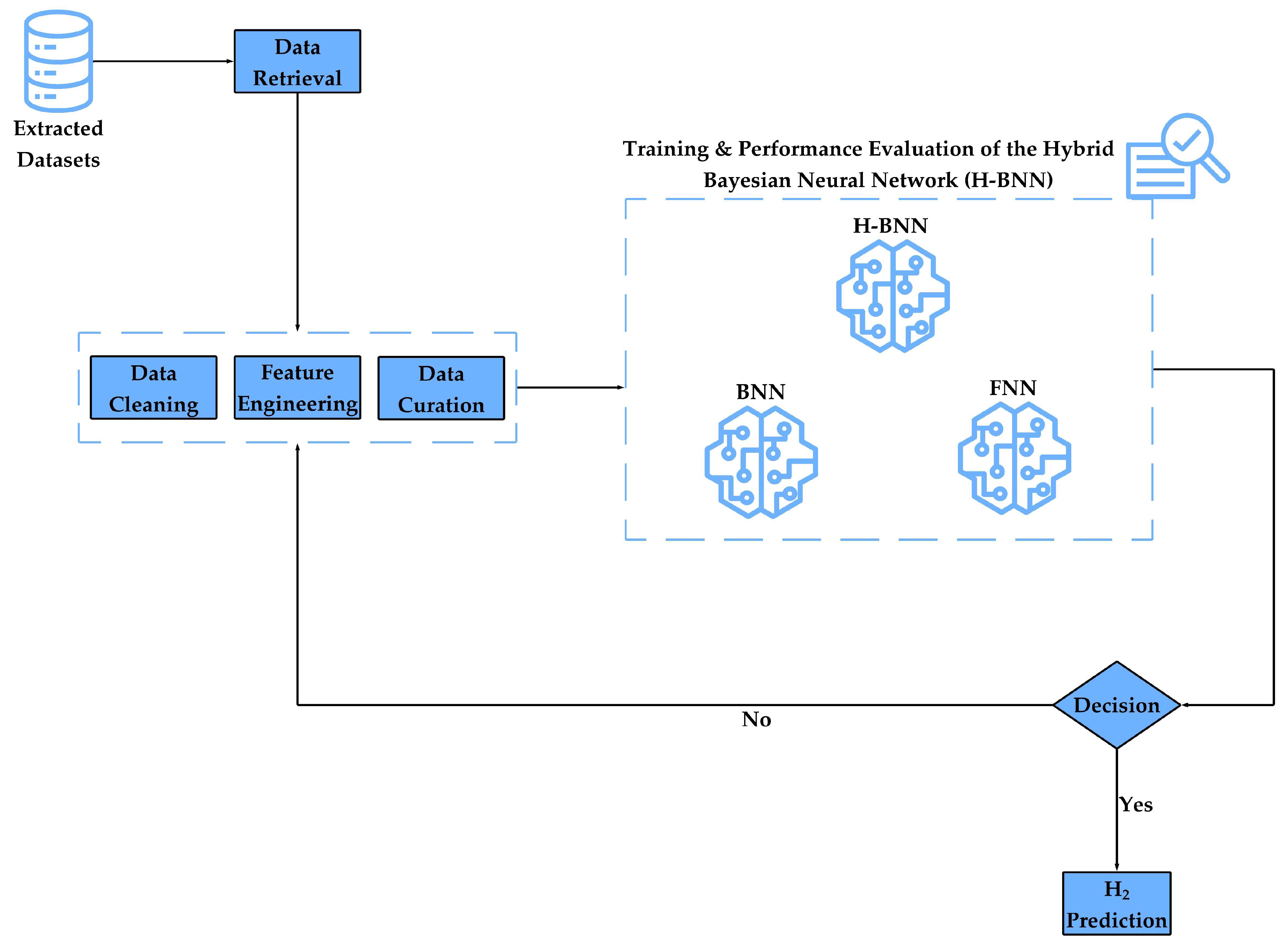
The mined datasets obtained from the literature, whose works were aligned with the study, were used to develop the proposed neural networks: hybrid BNN (or H-BNN), classic BNN, and FNN. As illustrated in Figure 5, the datasets were curated and prepared to train the models, as shown in the workflow. The prepared dataset was divided into ratios of 70%, 15%, and 15% for the Training, Validation and Testing sets. Code execution was carried-out on a local machine equipped with an Intel Core Ultra 7 155H processor (16 cores, 22 threads, up to 4.8 GHz), 32 GB LPDDR5x RAM, and an NVIDIA GeForce RTX 4050 GPU with 6 GB of dedicated memory. Furthermore, Google Colab was deployed using a PyTorch-based Python environment (Python 3.x), with gradient computations performed via automatic differentiation and GPU acceleration enabled via CUDA when available.

The hybrid Bayesian Neural Network (H-BNN) was trained on a dataset extracted from the literature (see Table 2), which originated from different experiments on steam methane reforming (SMR) via induction heating. In addition, the experimental designs for the respective referenced studies based on SMR were on different scales based on the information provided in Table 2, such as the length and diameter of the reactor and other important variables. Furthermore, in this study, six (6) most important variables—temperature (T), pressure (P), flow rate (F), hydrogen yield (Y), power input (p), and time on stream (TOS) were considered in the training of the H-BNN, as shown in Algorithm A1, MoH was considered the target variable for predicting hydrogen production in SMR. Moreover, as illustrated in the workflow in Figure 5, the classic Bayesian Neural Network (BNN) and Feedforward Neural Network (FNN) were deployed to serve as a “sanity check” on the proposed hybrid BNN.

The post-processed H-BNN results in

Table 8. Combined post-processed outputs of the Hybrid-Bayesian neural network (H-BNN) at data augmentation scales $k=2$, 5, and 10, showing true and predicted mass of hydrogen (MoH), hydrogen yield, and specific energy consumption (SEC).

S/N	MoHpred ($\times {10}^{-3}$ kg)	MoHpred ($\times {10}^{-3}$ kg)	${\mathbf{Y}}_{{\mathit{H}}_{\mathbf{2}}}^{\mathbf{true}}$ (%)	${\mathbf{Y}}_{{\mathit{H}}_{\mathbf{2}}}^{\mathbf{pred}}$ (%)	SECtrue (kWh kg−1 H2)	SECpred (kWh kg−1 H2)
augmentation factor, k = 2
1	0.0305	0.0342	64.94	72.79	5573.77	4972.39
2	0.0304	0.0335	124.12	137.88	2651.89	2387.39
3	0.0459	0.0422	139.51	143.43	1907.30	1855.16
4	0.0352	0.0340	102.80	104.10	3521.13	3477.09
5	0.0311	0.0320	69.75	70.86	3116.70	3068.18
augmentation factor, k = 5
1	0.0305	0.0338	64.94	71.97	5573.77	5029.45
2	0.0304	0.0342	124.12	138.61	2651.89	2374.80
3	0.0459	0.0422	139.51	143.97	1907.30	1848.20
4	0.0352	0.0336	102.80	104.10	3521.13	3477.62
5	0.0311	0.0318	69.75	70.76	3116.70	3072.50
augmentation factor, k = 10
1	0.0305	0.0334	64.94	71.22	5573.77	5082.29
2	0.0304	0.0345	124.12	138.46	2651.89	2377.40
3	0.0459	0.0423	139.51	144.01	1907.30	1847.67
4	0.0352	0.0333	102.80	103.94	3521.13	3482.38
5	0.0311	0.0322	69.75	70.83	3116.70	3069.27

MoH is reported in kg, yield in %, and SEC in kWh kg⁻¹ H₂.

further show that in addition to predicting MoH, other meaningful trends such as hydrogen yield and specific energy consumption (SEC) across the augmentation scales of $k=2$, 5, and 10 could also be obtained.

As shown in

Table 9. Model performance for H-BNN, FNN, and BNN based on a data augmentation scale factor of $k=2$. The MAE and MSE are measured in grammes (or $\times {10}^{-3}$ kg) and grammes² (or $\times {10}^{-6}$ kg²), respectively.

Model	Activation	MAE	MSE	R2
FNN	GELU	0.0190	0.0030	0.9940
BNN	Tanh	0.0270	0.0090	0.9810
H-BNN	GELU	0.0126	0.0014	0.9969

,

Table 10. Model performance for H-BNN, FNN, and BNN based on a data augmentation scale factor of $k=5$. The MAE and MSE are measured in grammes (or $\times {10}^{-3}$ kg) and grammes² (or $\times {10}^{-6}$ kg²), respectively.

Model	Activation	MAE	MSE	R2
FNN	Tanh	0.0190	0.0040	0.9920
BNN	Tanh	0.0310	0.0080	0.9810
H-BNN	Tanh	0.0207	0.0048	0.9894

and

Table 11. Model performance for H-BNN, FNN, and BNN based on a data augmentation scale factor of $k=10$. The MAE and MSE are measured in grammes (or $\times {10}^{-3}$ kg) and grammes² (or $\times {10}^{-6}$ kg²), respectively.

Model	Activation	MAE	MSE	R2
FNN	Tanh	0.0240	0.0060	0.9860
BNN	Tanh	0.0230	0.0040	0.9900
H-BNN	Tanh	0.0217	0.0038	0.9915

, the scaling factor k significantly impacted training performance. The H-BNN achieved the best trade-off compared to classic BNN and FNN models. This stems from H-BNN’s effective combination of FNN’s deterministic power and Bayesian uncertainty quantification, at lower computational cost than classic BNN.

Furthermore, as shown in

Table 12. Predicted mass of hydrogen (MoH) by different neural-network architectures for a scale factor of $k=2$. MoH is measured in grammes (or $\times {10}^{-3}$ kg).

S/N	True Value	FNN	BNN	H-BNN
Mass of Hydrogen (MoH)
1	0.043	0.044	0.042 ± 0.001	0.044 ± 0.001
2	0.033	0.034	0.033 ± 0.001	0.034 ± 0.001
3	2.178	1.994	1.844 ± 0.065	2.167 ± 0.159
4	0.040	0.043	0.042 ± 0.001	0.043 ± 0.001
5	0.034	0.034	0.034 ± 0.001	0.034 ± 0.001

Activation Functions: FNN → GELU, BNN → Tanh, H-BNN → GELU.

,

Table 13. Predicted mass of hydrogen (MoH) by different neural-network architectures for a scale factor of $k=5$. MoH is measured in grammes (or $\times {10}^{-3}$ kg).

S/N	True Value	FNN	BNN	H-BNN
Mass of Hydrogen (MoH)
1	0.043	0.045	0.043 ± 0.001	0.045 ± 0.001
2	0.033	0.034	0.034 ± 0.000	0.034 ± 0.000
3	2.178	1.957	1.853 ± 0.065	1.929 ± 0.117
4	0.040	0.041	0.041 ± 0.001	0.041 ± 0.001
5	0.034	0.034	0.034 ± 0.000	0.034 ± 0.001

Activation Functions: FNN → Tanh, BNN → Tanh, H-BNN → Tanh.

and

Table 14. Predicted mass of hydrogen (MoH) by different neural-network architectures for a scale factor of $k=10$. MoH is measured in grammes (or $\times {10}^{-3}$ kg).

S/N	True Value	FNN	BNN	H-BNN
Mass of Hydrogen (MoH)
1	0.043	0.043	0.044 ± 0.000	0.045 ± 0.001
2	0.033	0.033	0.034 ± 0.000	0.034 ± 0.001
3	2.178	1.897	1.946 ± 0.063	1.961 ± 0.107
4	0.040	0.041	0.040 ± 0.000	0.041 ± 0.001
5	0.034	0.034	0.034 ± 0.000	0.034 ± 0.001

Activation Functions: FNN → Tanh, BNN → Tanh, H-BNN → Tanh.

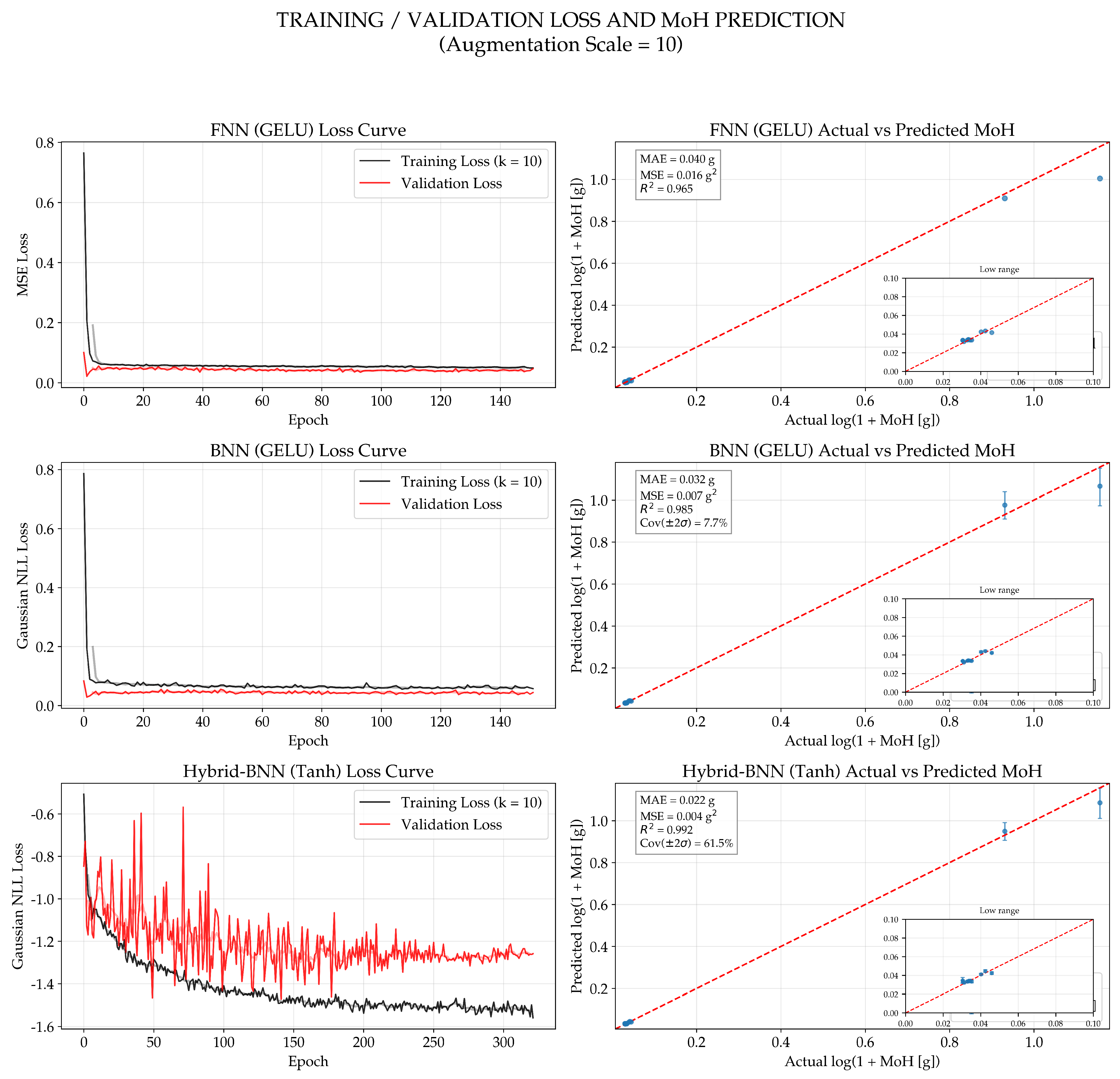
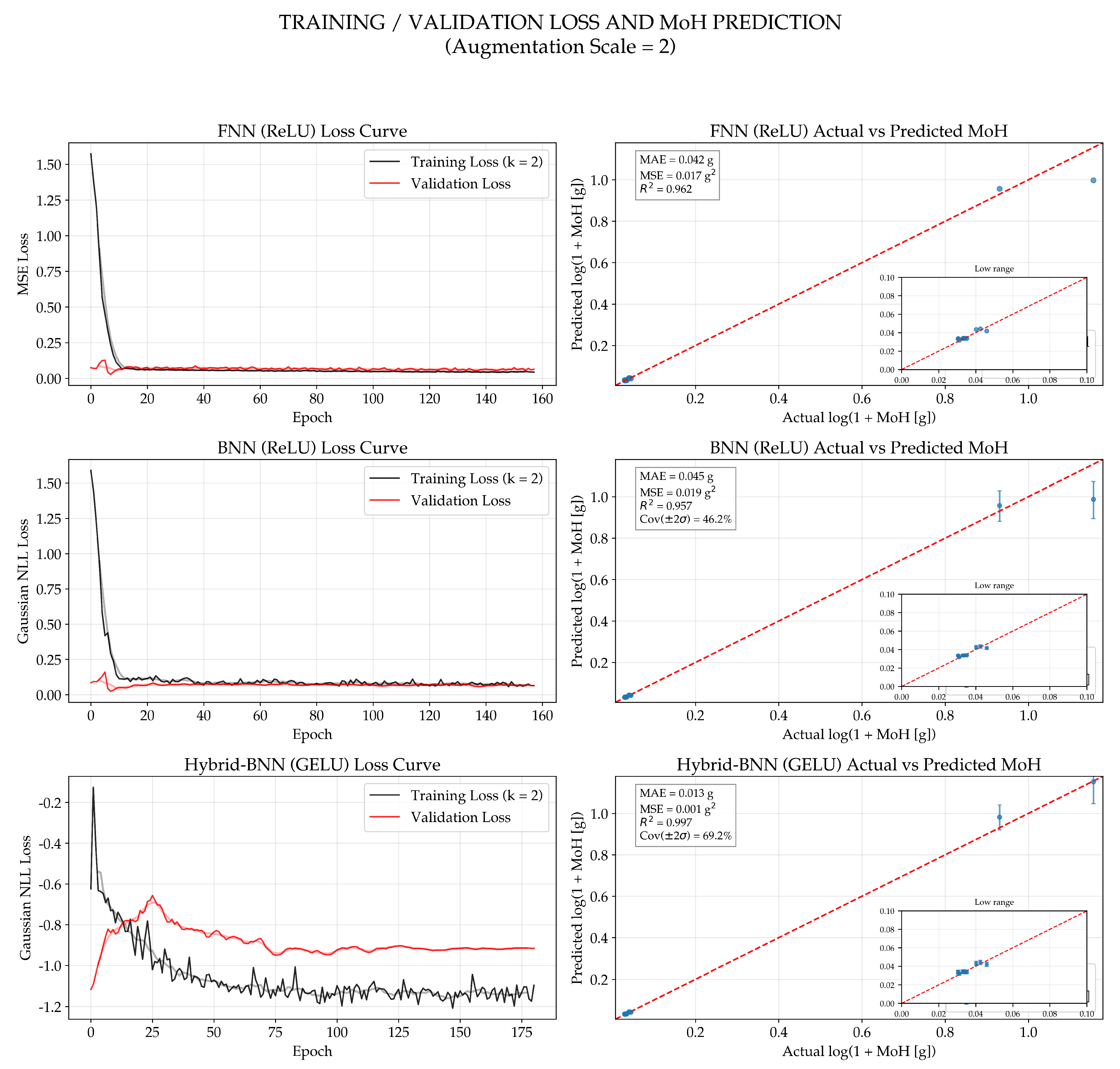
, the H-BNN, BNN, and FNN predictions of the hydrogen mass across the activation functions (GeLU, ReLU, and Tanh) highlight the predictive efficiency of H-BNN. Notably, reducing k from 10 to 2 reveals the capacity of H-BNN in terms of predictiveness and robustness within data-scarce scenarios, even with a training set of 70% of data points, balanced validation (15%), and test (15%) sets (See Figure 6, Figure 7 and Figure 8).

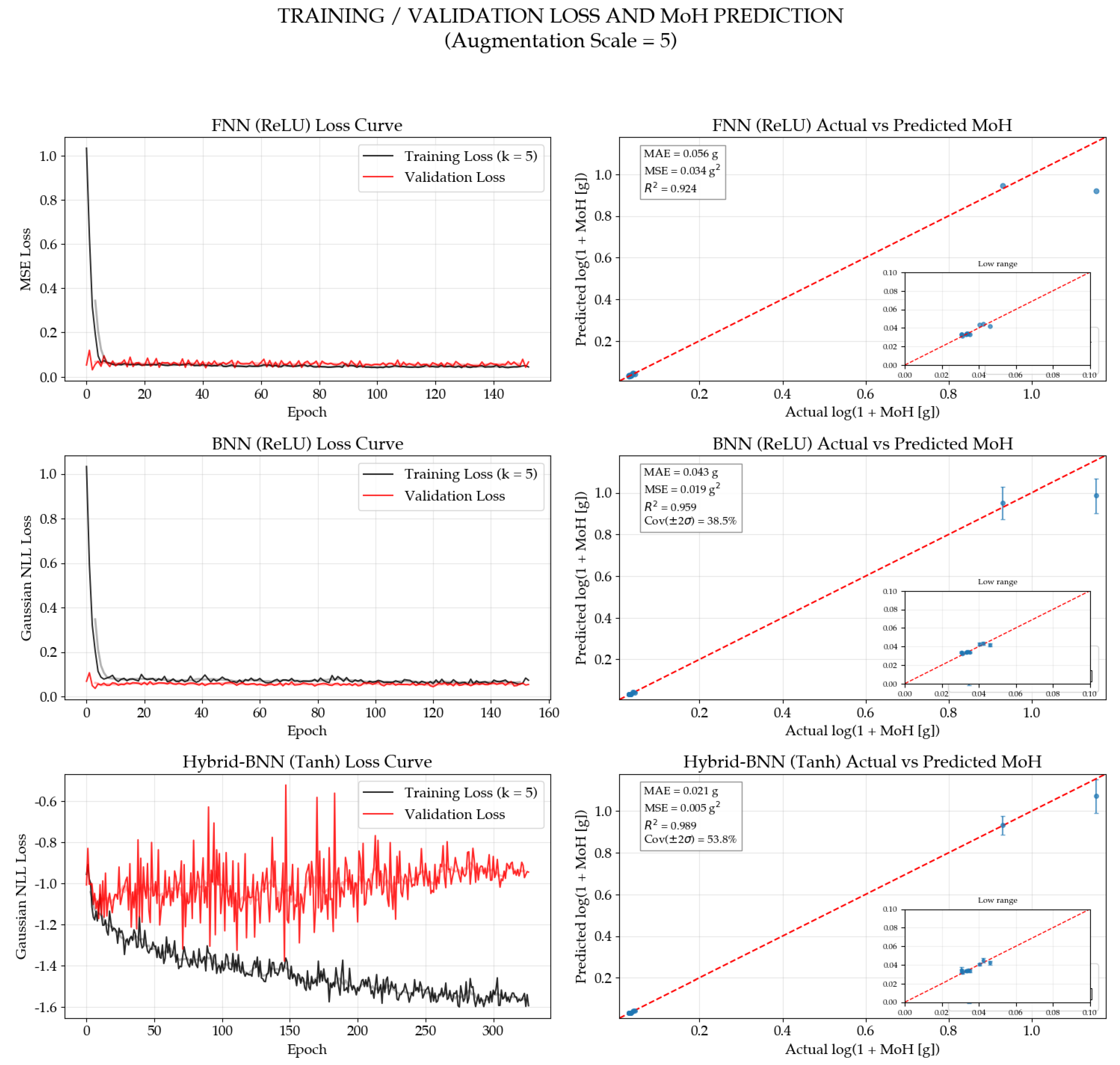
The graphical comparisons presented in Figure 6, Figure 7 and Figure 8 indicate that all three neural network models achieved rapid convergence during training. However, variations in convergence behavior and predictive quality were observed across different augmentation scales. Generally, the FNN and BNN demonstrated smoother and more stable loss trajectories, whereas the H-BNN exhibited a noisier negative log-likelihood profile, particularly at $k=5$ and $k=10$. This behavior aligns with the stochastic optimization characteristic of the H-BNN and the increased complexity of learning both the predictive mean and uncertainty structure from a limited dataset sourced from the literature. Nonetheless, the parity plots reveal that the H-BNN remained the most competitive architecture overall, with its most pronounced relative advantage manifesting under the lower-data condition at $k=2$.

At $k=2$, the H-BNN (GELU) demonstrated superior predictive performance among the models presented, achieving a mean absolute error (MAE) of $0.013$ g, a mean squared error (MSE) of $0.001$ g², and an $R^2$ value of $0.997$. In comparison, the FNN (ReLU) recorded values of $0.042$ g, $0.017$ g², and $0.962$, whereas the BNN (ReLU) exhibited $0.045$ g, $0.019$ g², and $0.957$, respectively. The parity plot for the H-BNN at this scale is notably closest to the ideal $1:1$ line, and the low-MoH inset further corroborates that the model maintained a high fidelity in the low-production region. Furthermore, the H-BNN achieved a $\pm 2\sigma$ coverage of $69.2\%$, which, although still below the nominal calibration, surpassed the corresponding BNN coverage of $46.2\%$. These findings suggest that the proposed H-BNN is particularly effective when the amount of augmented training information is limited.

At $k=5$, the comparative trend continued to favor the H-BNN, although the margin of improvement reduced. In the presented comparison, the H-BNN (Tanh) achieved a Mean Absolute Error (MAE) of $0.021$ g, a Mean Squared Error (MSE) of $0.005$ g², and an $R^2$ of $0.989$, surpassing the performance of the FNN (ReLU), which recorded $0.056$ g, $0.034$ g², and $0.924$, as well as the BNN (ReLU), which recorded $0.043$ g, $0.019$ g², and $0.959$. The parity plot for the H-BNN once again demonstrated the closest alignment with the ideal line, particularly for the higher MoH points, despite a noticeably noisier loss history. This indicates that the stochasticity observed in the H-BNN training curve did not result in a suboptimal predictive performance for the test set. However, the quality of uncertainty remained limited, with a $\pm 2\sigma$ coverage of $53.8\%$, suggesting that the predictive intervals were still under-calibrated despite the strong accuracy of point predictions.

At $k=10$, the H-BNN (Tanh) demonstrated superior performance among the models presented, achieving a Mean Absolute Error (MAE) of $0.022$ g, a Mean Squared Error (MSE) of $0.004$ g², and an $R^2$ value of $0.992$. In comparison, the FNN (GELU) recorded values of $0.040$ g, $0.016$ g², and $0.965$, whereas the BNN (GELU) achieved $0.032$ g, $0.007$ g², and $0.985$. Furthermore, the H-BNN exhibited the highest interval coverage at this scale, with a coverage of $61.5\%$, whereas the BNN (GELU) displayed significantly lower uncertainty performance, with only $7.7\%$ coverage. Despite the H-BNN’s loss curve being more irregular than those of the FNN and BNN, its parity plot and summary metrics confirmed its superior predictive performance among the models depicted in the figure.

The post-processed results of the H-BNN, as detailed in Table 8, further substantiate that the model successfully preserved physically meaningful trends in the predicted mass of hydrogen (MoH), hydrogen yield, and specific energy consumption (SEC) across the examined augmentation scales of $k=2$, 5, and 10. Notably, the predicted MoH values remained closely aligned with the corresponding true values for all cases, with only minor deviations observed across the three augmentation conditions. For instance, under the first operating condition, the true MoH of $0.0305$ g was predicted as $0.0342$ g, $0.0338$ g, and $0.0334$ g for $k=2$, 5, and 10, respectively, indicating a stable model response to the augmentation scale. Similarly, for the third operating condition, which corresponds to the highest MoH level among the listed cases, the H-BNN predicted $0.0422$ g, $0.0422$ g, and $0.0423$ g relative to the true value of $0.0459$ g, thereby demonstrating a consistent predictive behaviour even in the higher-production regime.

A comparable trend was observed for the hydrogen yield and specific energy consumption (SEC). The predicted hydrogen yield values were generally marginally higher than the corresponding actual values, indicating that the H-BNN could capture the anticipated production trend while slightly overestimating the conversion performance in certain instances. For instance, under the second operating condition, the actual hydrogen yield of $124.12\%$ increased to predicted values of $137.88\%$, $138.61\%$, and $138.46\%$ for $k=2$, 5, and 10, respectively. Concurrently, the SEC predictions were slightly lower than the actual values, suggesting that the model tended to predict more energy-efficient hydrogen production than that empirically observed. Notably, the predicted SEC for the fifth operating condition decreased from the actual value of $3116.70$ kWh kg⁻¹ H₂ to $3068.18$, $3072.50$, and $3069.27$ kWh kg⁻¹ H₂ for $k=2$, 5, and 10, respectively. Overall, the relatively minor variation in the post-processed outputs across the three augmentation scales suggests that the H-BNN maintained robust predictive consistency, with the strongest overall point-prediction performance still observed under the lower-data condition, particularly at $k=2$.

In general, graphical and numerical analyzes demonstrate that the H-BNN architecture exhibits superior competitiveness under conditions of reduced data, with its most pronounced relative advantage observed at $k=2$. Concurrently, the model maintained robustness across the examined augmentation scales and upheld physically coherent trends in MoH, hydrogen yield, and SEC. These results confirm the appropriateness of the H-BNN as a data-driven predictive framework for hydrogen-production modelling using limited and heterogeneous datasets derived from the literature.

5. Conclusions

This study introduces a hybrid Bayesian neural network (H-BNN) to predict hydrogen production from literature-derived datasets with limited, heterogeneous observations across experimental designs. The model was trained, validated, and tested on a curated dataset featuring key operating variables: temperature, flow rate, catalyst/bed loading, power input, and time on stream (TOS). These inputs enabled accurate mass of hydrogen (MoH) predictions. The H-BNN delivered robust point predictions across augmentation scales. Moreover, data augmentation improved generalization, with H-BNN showing the greatest relative advantage under low-data conditions, particularly at k = 2 as discussed previously.

The procedure for deploying the H-BNN model is described in detail. Across the evaluated augmentation scales, the H-BNN achieved high predictive accuracy, with $R^2$ values of approximately 0.997, 0.989, and 0.992 for $k=2$, $k=5$, and $k=10$, respectively, for the validation-selected models. Correspondingly, the model yielded MAE values of 0.0126 g, 0.0207 g, and 0.0217 g, respectively, which correspond to errors on the order of ${10}^{-5}$ kg. These results affirm that the proposed H-BNN is highly effective for hydrogen-production prediction under data-scarce conditions, particularly when compared with the benchmark FNN and BNN models. However, although the H-BNN improved the predictive uncertainty representation relative to the classical BNN, the uncertainty intervals remained below the nominal calibration across the investigated cases and should thus be interpreted as informative, rather than fully calibrated.

Finally, the Monte Carlo dropout component in the H-BNN model captures the predictive uncertainty, providing a valuable basis for robust data-driven inference. The post-processed results further demonstrated that the H-BNN was capable of recovering physically meaningful trends not only in MoH but also in hydrogen yield and specific energy consumption (SEC), as shown in Table 8. Accordingly, depending on the nature and size of the available dataset, the proposed model has the potential to be extended to predict other output variables, such as SEC and emission-related indicators, in the context of steam methane reforming powered by induction heating.