Robust Optimisation of an Online Energy and Power Management Strategy for a Hybrid Fuel Cell Battery Shunting Locomotive

Abstract

Shunting locomotives exhibit a wide and unpredictable range of power profiles. This unpredictability makes it impossible to rely on offline optimizations or predictive methods combined with online optimization. To maintain optimal performance across this broad range of operating conditions, the online control strategy must be robust. This article proposes a robust method to determine the optimal parameter combinations for an online energy management strategy of a hybrid fuel cell battery shunting locomotive, ensuring optimality across all scenario conditions. The first step involves extracting a statistically representative subspace for simulation, both in terms of parameter combinations and scenario conditions. A response surface model (numerical twin) is then constructed to extrapolate results across the entire space based on this simulated subspace. Using this model, the optimal solution is identified through metaheuristic algorithms (minimization search). Finally, the proposed solution is validated against a set of expert-defined scenarios. The result of the methodology ensures robust optimization across an infinite number of scenarios by minimizing the impact on both the fuel cell and the battery, without increasing mission costs.

1. Introduction

The fuel cell (FC) and Li-ion battery hybrid train has a significantly higher cost than other propulsion systems, such as diesel or battery-only configurations. The analysis in [1] presents the Total Cost of Ownership (TCO) of a hydrogen train compared to battery and diesel trains in the USA. FC trains are estimated to be 13% more expensive, with a cost of USD 20.51/km, compared to USD 18.06/km for full battery trains and USD 18.01/km for diesel trains. Moreover, the FC cost assumptions in this analysis are optimistic—USD 193/kW—whereas the actual price of Proton Exchange Membrane Fuel Cells (PEMFC) was around USD 1800/kW in 2019, according to [2]. A more recent study [3] (2023) on 100 kW PEMFC prices for maritime applications (comparable to railway FC) reports costs ranging from USD 2278/kW for small-scale production (100 units/year) to USD 1652/kW for large-scale production (50,000 units/year). Reducing the TCO is therefore a key objective.

Shunting locomotives are primarily used to move wagons between trainsets. Unlike passenger transport, where missions are relatively predictable (with variations in passenger load that can be forecasted using learning methods such as peak hours or events), shunting operations are highly variable. Tasks can range from moving wagons on flat terrain to navigating humping hills for sorting, with loads varying from tenths to thousands of tons. This variability makes offline optimization methods, such as Dynamic Programming (DP) [4,5], impractical. Even online optimization approaches like [6] are not feasible due to the unpredictability of the locomotive’s next task.

As a result, Energy and Power Management Systems (EPMSs) are limited to rule-based control strategies, such as fuzzy logic. However, even in these cases, optimizing the membership functions requires tailoring to specific profiles, as shown in [7,8,9], not matching the wide variety of scenarios. The locomotive fuel cell system is designed as a range extender, and its missions can vary from light tasks involving only a few tons to demanding operations involving thousands of tons. To address this variability, the energy management strategy is based on a power moving average, like the EMS developed in [10]. This moving average is combined with a state machine, as presented in [11,12], to ensure that when the battery SOC (state of charge) is low, the FC operates at maximum power, and when the battery SOC is nearly full, the FC reduces power or shuts down.

This rule-based strategy must be optimized to reduce the high TCO of the locomotive. The method for optimizing such an EPMS is presented in this article. Monte Carlo methods, such as those used to generate scenarios in [13], are too computationally intensive due to the vast number of scenarios that must be tested. The Taguchi method is promising for estimating the impact of parametric noise [14,15], but it does not account for the probability of occurrence of each scenario condition—such as the likelihood of the battery’s state of energy (SOE) being near the EPMS target.

An overview of the proposed method is presented in Section 3.1. The first step (Section 3.2.2) involves selecting a subspace of scenarios based on the probability of occurrence of each condition (e.g., wagon load, temperature, initial SOE). A representative set of parameter combinations is selected to cover the parameter space (Section 3.2.1), and all selected scenarios are simulated. A response surface model (RSM) is then trained on the simulation results (Section 3.3.2) to predict outcomes for unsimulated parameter combinations. Each combination is scored based on performance (ensuring locomotive functionality is not compromised) and TCO (Section 3.3.1). The optimal score is identified using optimization algorithms, such as the metaheuristics presented in [7,8,9] (Section 3.3.3). Finally, the optimal solution is validated on a set of scenarios defined by the locomotive specifications (Section 3.3.4).

2. Modelling

The simulation tool used for calculations is an Alstom’s internal tool. While the global physical principles and modeling approach will be partially detailed in the following sections, the focus will be on the development of the longitudinal dynamics model, followed by a discussion of the electrical components of the traction drive.

2.1. Longitudinal Dynamics Model

The longitudinal dynamics are modeled using Equation (1),

$$M^{*}. \Gamma =F_{motors}+F_{brakes}+F_{RTM}+F_{weight}+F_{curves}$$

(1)

$$M^{*}=M_s+M_T$$

(2)

where $\Gamma$ is the train acceleration in m/s². $M^{*}$ is the dynamic mass of the train, defined by Equation (2), and it is composed of the static mass $M_s$ (empty train mass + load mass) and $M_T$, the rotating mass in kg given by Equation (3).

$$M_T=\sum \left({\displaystyle \frac{J_e}{R^2}}+{\displaystyle \frac{J_r{\rho }^2}{R^2}}\right)$$

(3)

where $J_e$ is the moment of inertia of rotating masses on powered or non-powered axles, in kg.m². $J_r$ is the moment of inertia of rotating masses on the motor axles, in kg.m². R is the wheel radius in m. $\rho$ is the gear ratio (motor speed/wheel speed > 1).

$F_{motors}$ is the effort provided by the motors (traction and electrodynamic braking), in N.

$F_{brake}$ is the effort provided by the mechanical brake, in N.

$F_{RTM}$ is the resistance to motion, defined using a modified Davis formula, such as in Equation (4),

$$F_{RTM}=A+B.V_{train}+C.T_f.\left(V_{train}-V_{wind}\right).|V_{train}-V_{wind}|$$

(4)

The A, B and C coefficients are the resistance to motion coefficients expressed respectively in N, N/(km/h) and N/(km/h²). The C coefficient depends on the temperature and altitude of the train. $V_{wind}$ is the longitudinal component of the wind in km/h. Finally, $T_f$ is the tunnel factor, which increases aerodynamic resistance in tunnels and depends on tunnel length and cross-section.

$F_{weight}$ is the gravitational component due to track slope, given by Equation (5),

$$F_{weight}=M_s . g .\sin \left(\alpha \right)\approx M_s . g .\tan \left(\alpha \right)=M_s . g . grad$$

(5)

where $\alpha$ is the angle of the slope (assumed small, consistent with railway constraints) and $grad$ is the slope gradient, in o/oo.

$F_{curves}$ is the resistance due to track curvature, given by the Rockl formula (Equation (6)),

$$F_{curves}={\displaystyle \frac{K}{(R-R_r)}} . M_s . g$$

(6)

where k is the resistance in the curve coefficient in N/kg.m and $R_r$ is the Rockl correction factor in m.

Finally, R is the curve radius in m.

The simulation tool has been in use for several years, and its results have been correlated. An example of the output generated by the tool is shown in Figure 1.

2.2. Traction Drive Model

The train consists of two independent traction drives, each featuring a hybrid parallel architecture combining a fuel cell and a battery. Both the FC and the energy storage unit (ESU) are connected to the DC bus via their own dedicated step-up chopper. In addition, inverters and an auxiliary converter are also connected to the same DC bus. The schematic of the electrical architecture is shown in Figure 2.

The traction equipment, which includes the inverter, motor, and gearbox, is modeled using power loss maps. The step-up choppers are also represented through similar power loss maps.

The sources, FC and ESU, are modeled as black boxes, based on data provided by the suppliers.

An average auxiliary load is applied to account for auxiliary power consumption. This average load is estimated using a separate tool that considers different ambient temperatures. However, the auxiliaries of the FC and the ESU are excluded from this average value because they are already calculated by their respective models. The auxiliaries of the FC and ESU are composed of their cooling system and their electronic control. Besides this, the FC has additional auxiliaries such as the air blower and H₂ pump.

The FC ageing model is based on a static model from [16], which maps FC degradation (in µV/h) to its operating point. The model defines distinct operating ranges, such as low power, galvanostatic, and high power, each associated with a specific degradation rate. The extent of damage depends on the power range in which the FC is operating.

The EPMS used in this study will combine a state-based control law such as [11,12] with a range extender mode. Depending on the battery’s SOE, the fuel cell power setpoint will be fixed. However, in one specific region, referred to as the nominal region, the power setpoint will be determined as the moving average over a defined past time window similar to [10]. This approach is called the range extender mode, which will be explained in more detail in Section 3.2.1. The control law is illustrated in Figure 3.

3. Optimization Methodology

The shunting locomotive may undertake a wide variety of missions throughout its lifetime. The energy management parametrization needs to ensure optimality for all possible scenarios. In this section, we present a robust optimization methodology.

3.1. Overview

The methodology consists of several key steps. Before applying it, it is essential to define the complete DoE (design of experiment) space. This involves identifying all relevant EPMS parameters and their respective ranges to define the EPMS parameter space. Similarly, all potential operational scenarios must be identified, along with their occurrence probabilities, to define the scenario space.

Since simulating the entire parameter and scenario spaces is computationally infeasible, the first step of the method aims to reduce the number of simulations. This is achieved by selecting a representative and homogeneous subset of points from both the EPMS parameter space and the scenario space. For the EPMS parameter space, we begin with 100 points, as this space will later be used to train machine learning models. For the scenario space, 30 representative scenarios will be selected. This reduced scenario set ensures robustness by covering a wide variety of cases, weighted by their occurrence probabilities.

Each combination of EPMS parameters will be simulated across all selected scenarios (resulting in 3000 simulations). A cost function will be applied to each scenario simulation for a given parameter set, and the expected cost will be computed for each of the 100 parameter combinations.

The target of 3000 simulations was set deliberately. Based on our estimates, this number of simulations could be completed in under one day using our simulation tool, making execution speed a key factor. To reach this threshold, a sufficiently large number of EPMS parameter combinations is required to effectively train the model. To ensure robustness, the Taguchi method requires 13 simulations (2n + 1) for 6 scenario conditions. However, to further enhance robustness, this number must be at least doubled.

This provides a mapping of each EPMS parameter set to its expected performance across the scenario space. A machine learning model can then be trained to approximate this response surface. Using this model, we can identify the global minimum of the expected cost function over the scenario space.

Finally, the optimal parameter set obtained will be validated against a separate set of scenarios. These validation scenarios are selected by experts and customers to be representative of real-world operations.

The entire methodology is illustrated in Figure 4.

3.2. Study Design of Experiment

The online energy management strategy presented previously includes several tunable parameters, which will be defined and their application domain given in the following section.

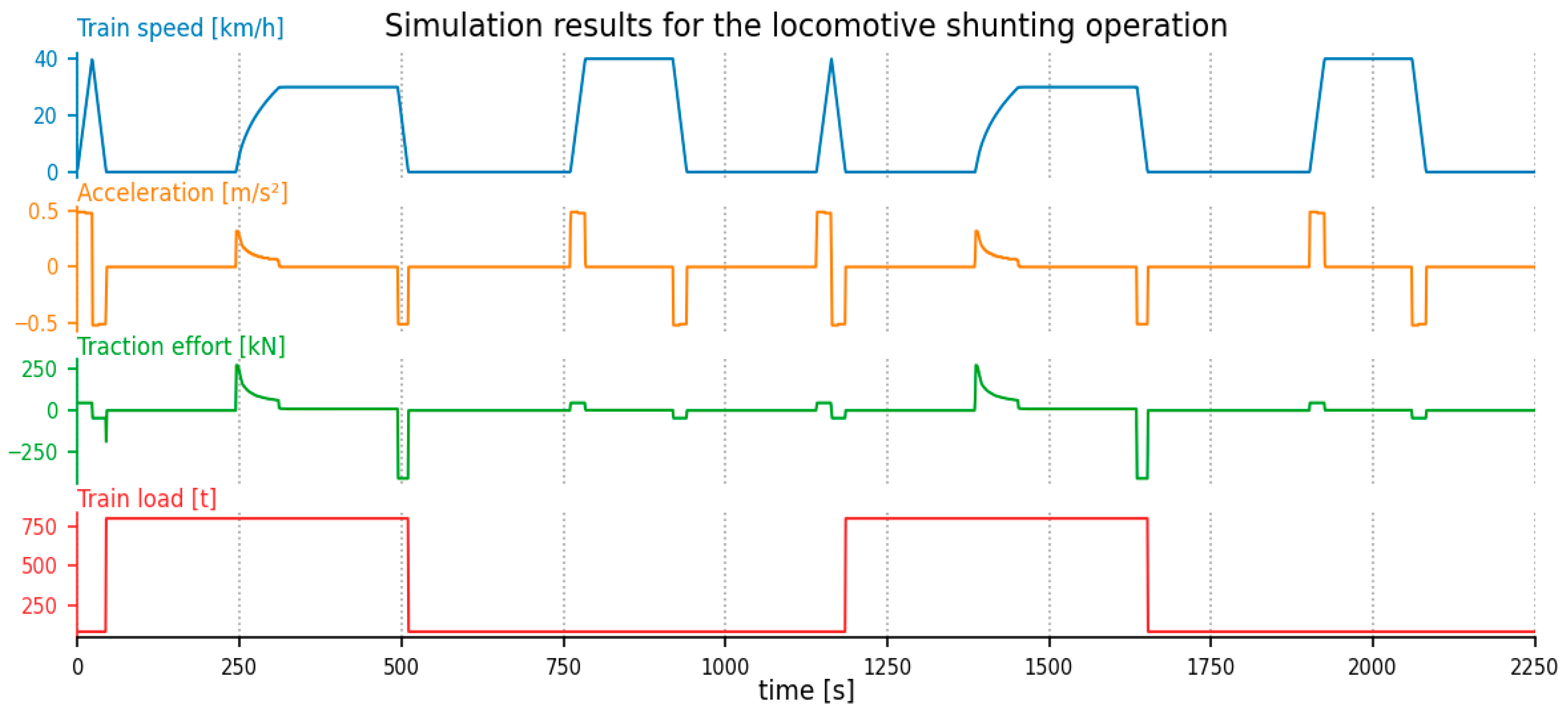
As already mentioned, the shunting locomotive may be assigned a wide variety of missions. For instance, the weight of the wagons it hauls can range from a few hundred tons up to 2000 tons, as is the case for the locomotive under study. Moreover, the load hauled is often unpredictable. The diversity and randomness of these missions necessitate a robust energy management system capable of handling the full range of operational scenarios to ensure optimal locomotive performance.

3.2.1. EPMS Parameters

The range extender (RE) mode’s objective is to maintain the battery energy level near the nominal threshold, but without abrupt changes. To achieve this, the system considers the recent power demand, as follows:

A long-term regulation where the objective is to recharge the battery to a nominal energy level. The next terms are demand oriented.

A medium-term average (shorter than the time required to reach the nominal energy threshold) is used to assess the general power demand trend.

A shorter-term average is also considered to allow for a more dynamic response to sudden changes in demand.

This dual-timescale approach helps the system balance energy stability and responsiveness. Equation (7) summarizes the logic of the range extender mode.

$$P_{FC}\left(t\right)={\displaystyle \frac{E_{nominal}-E_{bat}\left(t\right)}{T_{long}}}+{\displaystyle \frac{{\alpha }_{medium}}{T_{medium}-T_{short}}}{\int }_{t-T_{medium}}^{t-T_{short}}{P}_{need}\left(t\right).dt+{\displaystyle \frac{{\alpha }_{short}}{T_{short}}}{\int }_{t-T_{short}}^t{P}_{need}\left(t\right).dt$$

(7)

Let $P_{FC}$ be the power setpoint for the fuel cell, and $P_{need}$ the total power demand, which includes both auxiliary consumption and traction/braking consumption. Let $E_{nominal}$ and $E_{bat}$ represent the battery energy levels at the nominal threshold and the current state of charge, respectively. The parameters $T_{long}$, $T_{medium}$ and $T_{short}$ are time windows used for averaging power demand, while ${\alpha }_{medium}$ and ${\alpha }_{short}$ are weighting coefficients. These five parameters are subject to tuning as part of the energy management strategy.

The energy thresholds were defined during the system sizing phase to match the mission profiles established for the project. The five parameters mentioned above remain to be optimized. They are subject to constraints, which are summarized in the following Equations (8)–(11):

$${30\mathrm{s}<T}_{short}<T_{medium}<T_{long}<2\mathrm{h}$$

(8)

$${\alpha }_{short}+{\alpha }_{medium}=1$$

(9)

$$0\le {\alpha }_{short}\le 1$$

(10)

$$0\le {\alpha }_{medium}\le 1$$

(11)

The number of possible combinations is too high (>10¹⁰ with duration step of 30 s and ratio step of 1%). Simulating every combination is therefore computationally infeasible. We need to significantly reduce the number of combinations. While the Taguchi method could be considered, our goal is not to analyze parameter sensitivity but rather to train a machine learning (ML) model. To ensure the generalizability of the model, it is essential to sample the parameter space uniformly and comprehensively. Latin Hypercube Sampling (LHS) will be used. 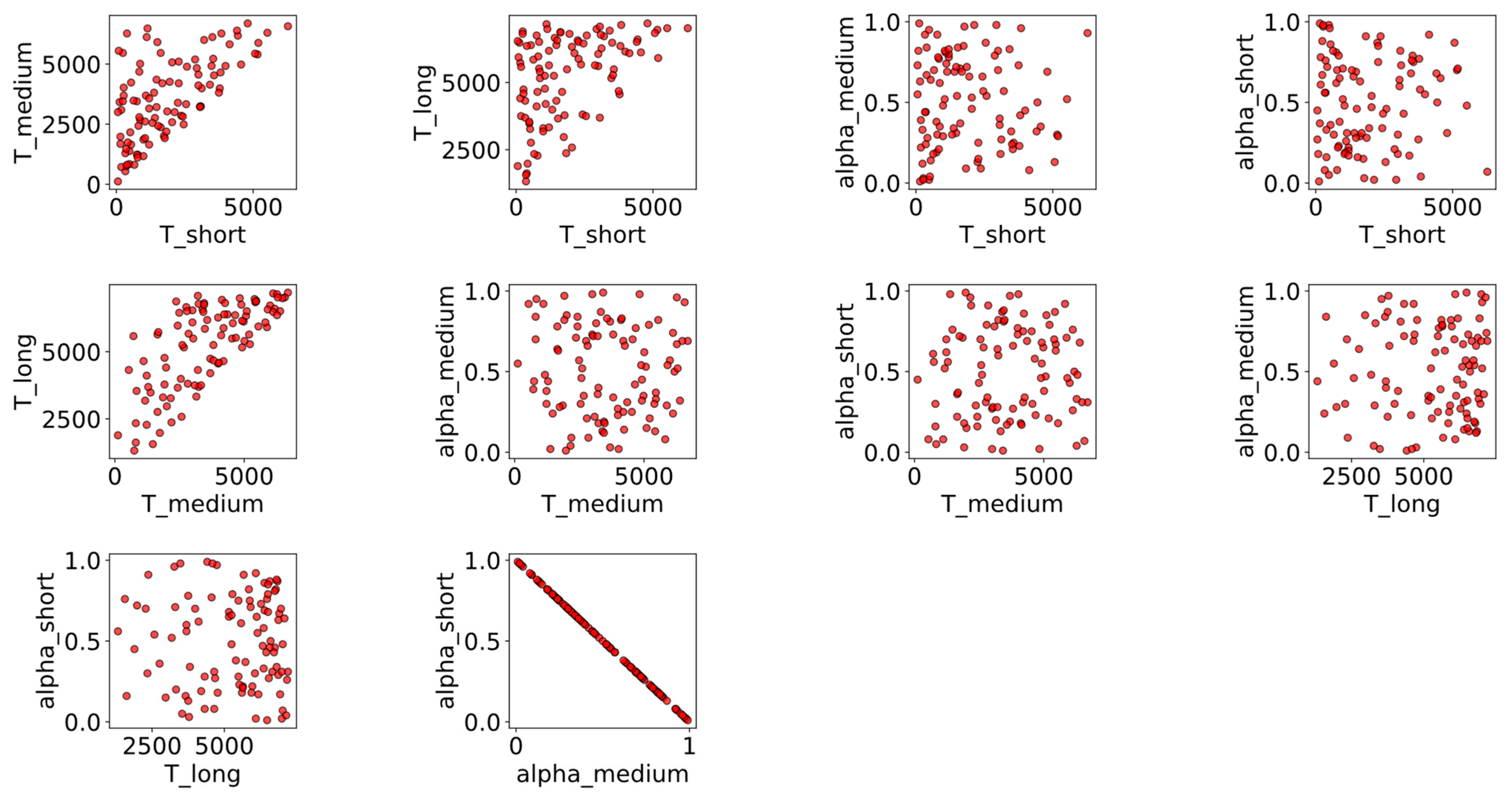This is a statistical method designed to ensure the even coverage of the parameter space [17]. Thanks to the LHS, the number of parameter combinations can be reduced to 100 for the initial phase. This number is sufficient to begin training the ML model. The representation of the selected combinations is given on Figure 5.

We observe that with only 100 points distributed across five constrained dimensions, the sampling appears visually to cover the entire constrained space relatively evenly.

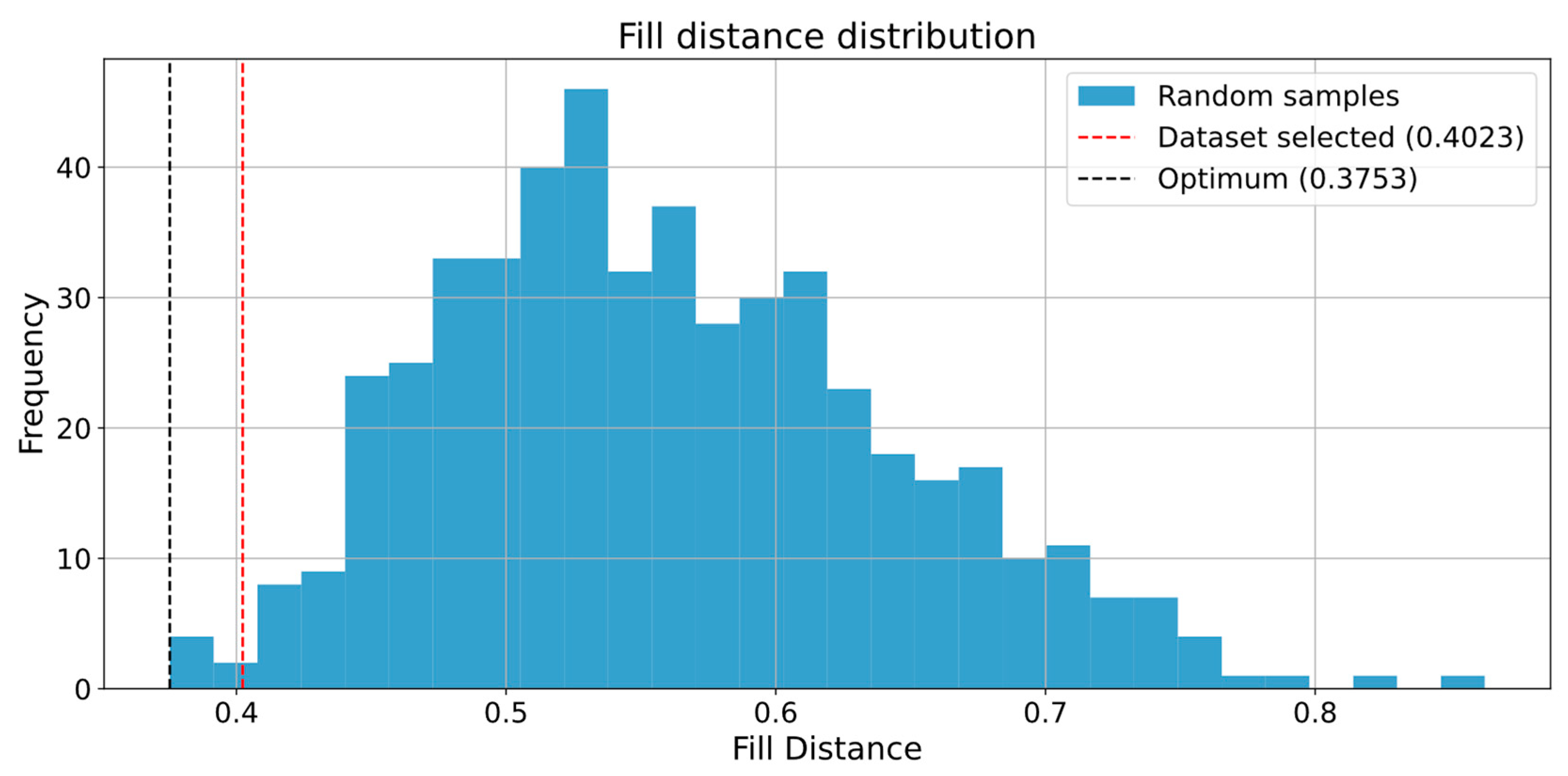
To estimate whether this dataset sufficiently covers the 5D constrained space, we compute the maximum distance from any point in the space to the nearest of our 100 sampled points. In a normalized 5D space, the theoretical maximum distance is $\sqrt{5} \approx 2.24$. In our case, the observed maximum distance is 0.4, which represents approximately 18% of the theoretical maximum. This suggests a good level of coverage.

To further assess this, we compare our result to 500 random draws of 100 points within the same 5D constrained space. The results are shown in Figure 6. We can observe that the selected solution is very close to the optimum (0.4 vs. 0.38). This indicates that the coverage achieved with thew 100 points sampled from our 5D constrained space is nearly optimal.

3.2.2. Scenario Conditions

To ensure the robustness of the optimization process, it is not sufficient to optimize all parameters based on a single scenario. The optimization must account for the full range of possible scenario conditions. These conditions include:

• Mission type;
• Train load;
• Ambient temperature;
• State of Health (SOH) of the FC and the ESU;
• Battery’s initial SOE;
• Average power initialization.

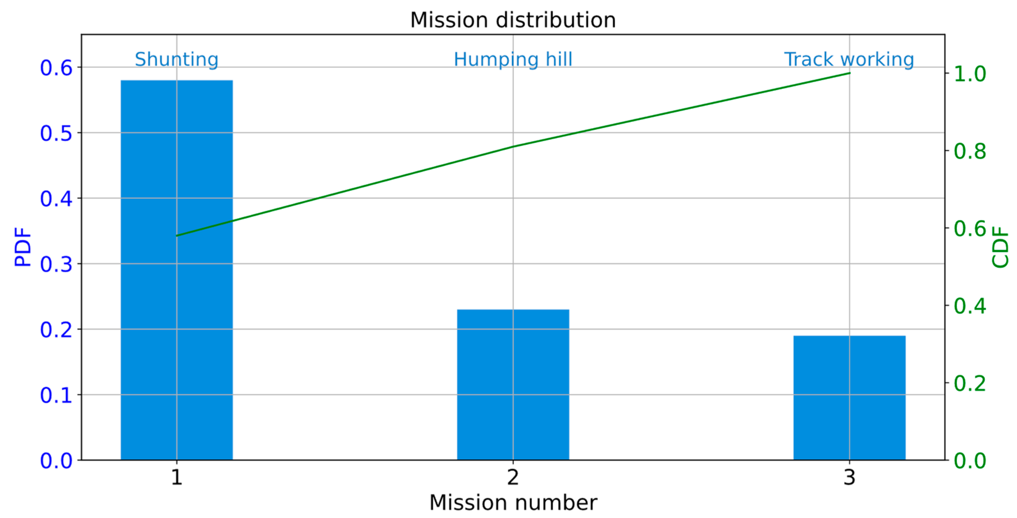
For the locomotive study, three representative missions have been selected:

• Shunting Mission

In this mission, the locomotive retrieves wagons of varying loads. The train runs empty in one direction and fully loaded in the other, with the load ranging from 500 to 2000 tons. This round trip is repeated 10 times consecutively;

2.

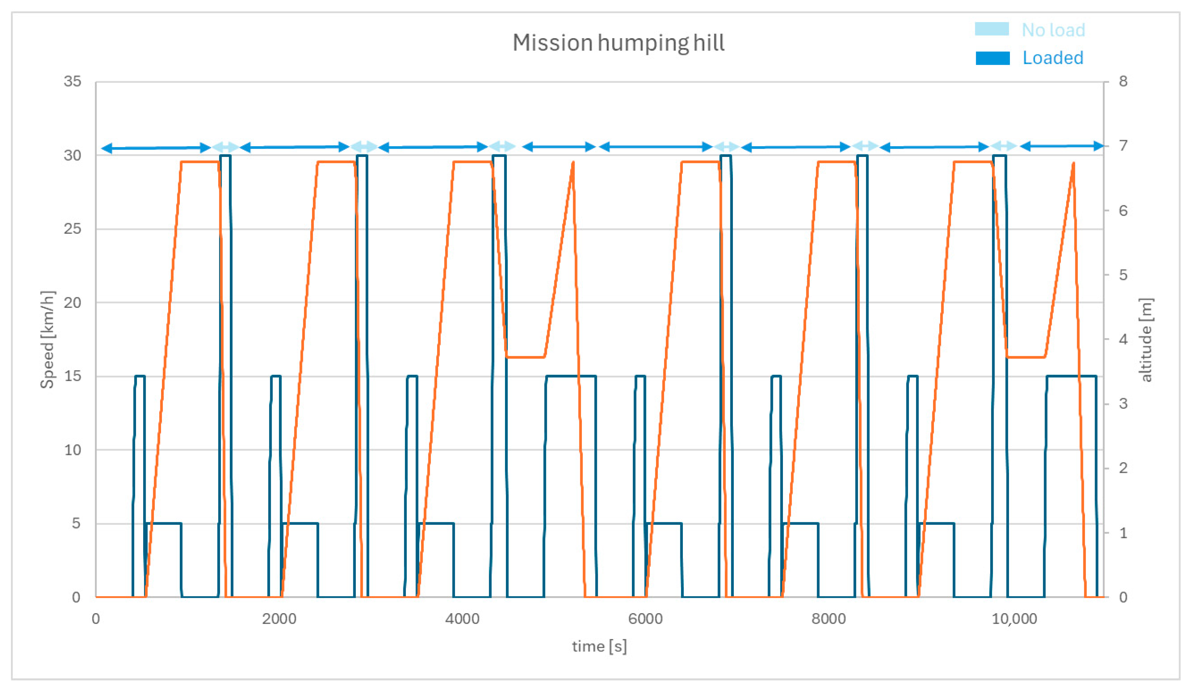
Humping Hill Mission

The locomotive pushes wagons to the top of a humping hill and then releases them. As with the previous mission, the load can vary between 500 and 2000 tons. The potential energy gained at the summit is used to sort the wagons;

3.

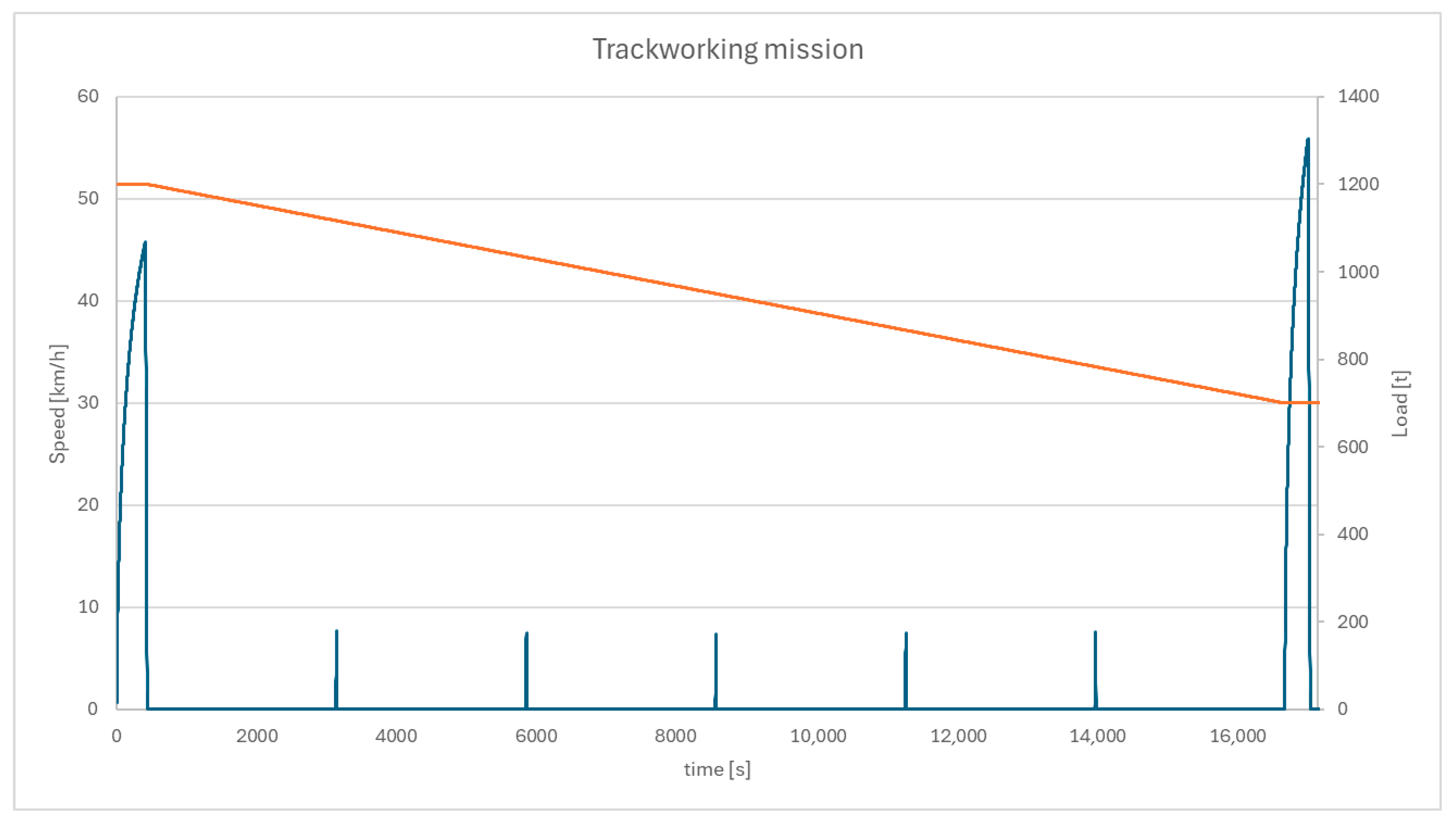
Track Work Mission

This mission simulates the locomotive towing a maintenance machine for track operations. It involves short back-and-forth movements. The convoy weighs approximately 1200 tons at the start, and after using materials for track repairs, the return trip weight is reduced to around 800 tons.

Figure 7 illustrates the Probability Density Function (PDF) and the Cumulative Density Function (CDF) associated with the mission occurrence.

For the wagon mass load, the locomotive is specified to carry up to 2000 tons. For the purpose of the study, we will use the wagon definition as given in the

Table 1. Wagon parameter definition.

Static Mass	Rotating Mass	Length	A	B	C
55 tons	800 kg	15 m	478.5 N	0 N/kph	0.1006 N/kph2

. When the loaded mass changes, other characteristics of the train also change resistance to motion, train length and mechanical brake effort. Each wagon adds its own resistance to motion and length to the convoys. Besides this, each wagon also has brake disks to help with mechanical braking.

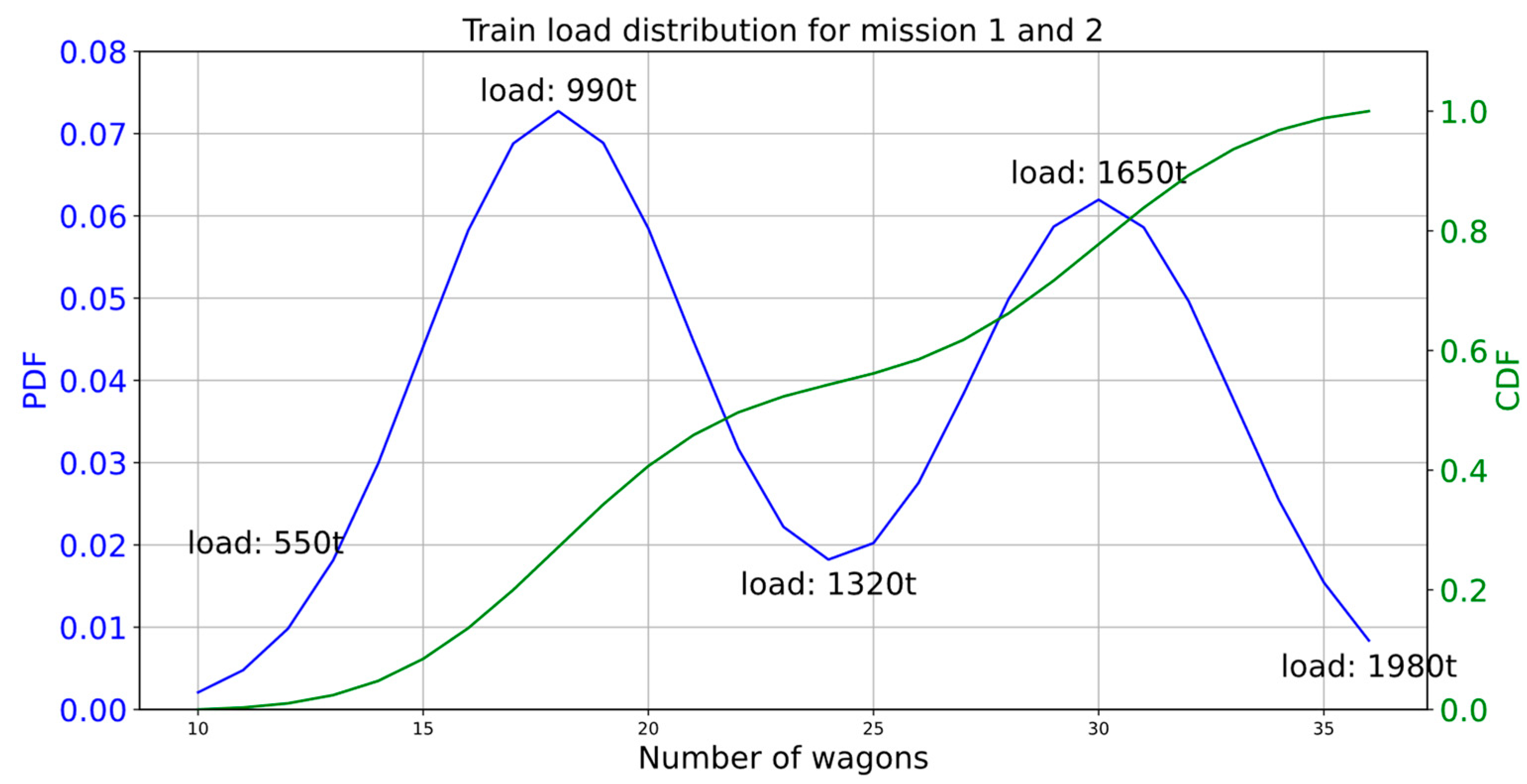
The shunting missions operate from 10 wagons up to 36 wagons. From the data of a customer, it appears that the most likely situations are around 1000 t (≈18 wagons) and between 1800 tons and 2000 tons (≈33 wagons). To represent the bimodal law, we have added two normal laws centered around 18 wagons and 30 wagons. The second peak for 30 wagons was a bit shifted to include a high density at 33 wagons, but a wider impact. This bimodal law is finally truncated between 10 wagons and 36 wagons. The bimodal probability density law is given by Equations (12)–(16) below.

$$P\left(X=x\right)=f\left(x, \mu ,\sigma \right)=\varphi \left( x, \mu , \sigma \right)$$

(12)

$$\varphi \left(x,\mu ,\sigma \right)={\displaystyle \frac{1}{\sqrt{2\pi {\sigma }^2}}} e^{-{\displaystyle \frac{{\left(x-\mu \right)}^2}{2{\sigma }^2}}}$$

(13)

Let $P\left(X=x\right)$ be the probability of X being x. We want to follow a normal distribution, with $\mu$ as the mean and $\sigma$ the standard deviation. The probability density function is then defined by Equation (13). The cumulative density function is then described by Equations (14) and (15).

$$P\left(X\le x\right)={\int }_0^{x}f(x,\mu ,\sigma )=F\left(x,\mu ,\sigma \right)=\Phi \left({\displaystyle \frac{x-\mu }{\sigma }}\right)$$

(14)

$$\Phi \left(z\right)={\displaystyle \frac{1}{2}} (1+{\displaystyle \frac{2}{\sqrt{\pi } }} {\int }_0^z{e}^{-{\displaystyle \frac{z^2}{2}}} dt)$$

(15)

$$PD{F}_{Train load}\left(x\right)={\displaystyle \frac{{\beta }_1. \varphi \left(x, {\mu }_1,{\sigma }_1\right)+{\beta }_2. \varphi \left(x, {\mu }_2,{\sigma }_2\right)}{\left[{\beta }_1 . \Phi \left(\frac{b-{\mu }_1}{{\sigma }_1}\right)+{\beta }_{2 }. \Phi \left(\frac{b-{\mu }_2}{{\sigma }_2}\right) \right]-\left[{\beta }_1 .\Phi \left(\frac{a-{\mu }_1}{{\sigma }_1}\right)+{\beta }_{2 }. \Phi \left(\frac{a-{\mu }_2}{{\sigma }_2}\right)\right]}}$$

(16)

$PD{F}_{Train load}\left(x\right)$ is the probability of having x wagons. ${\mu }_1$ and ${\mu }_2$ are the means of the two normal laws of the bimodal law. ${\sigma }_1$ and ${\sigma }_2$ are the standard deviations of the two normal laws of the bimodal law. Finally, both densities are not evenly distributed, and this distribution is represented by the parameters ${\beta }_1$ and ${\beta }_2$. Finally, the values are given in

Table 2. PDF for train load parameters.

${\mathit{\beta }}_1$	${\mathit{\mu }}_1$	${\mathit{\sigma }}_1$	${\mathit{\beta }}_1$	${\mathit{\mu }}_1$	${\mathit{\sigma }}_1$
0.54	18	3	0.46	30	3

. The graphic representation of the probability law for the mass load is given in Figure 8.

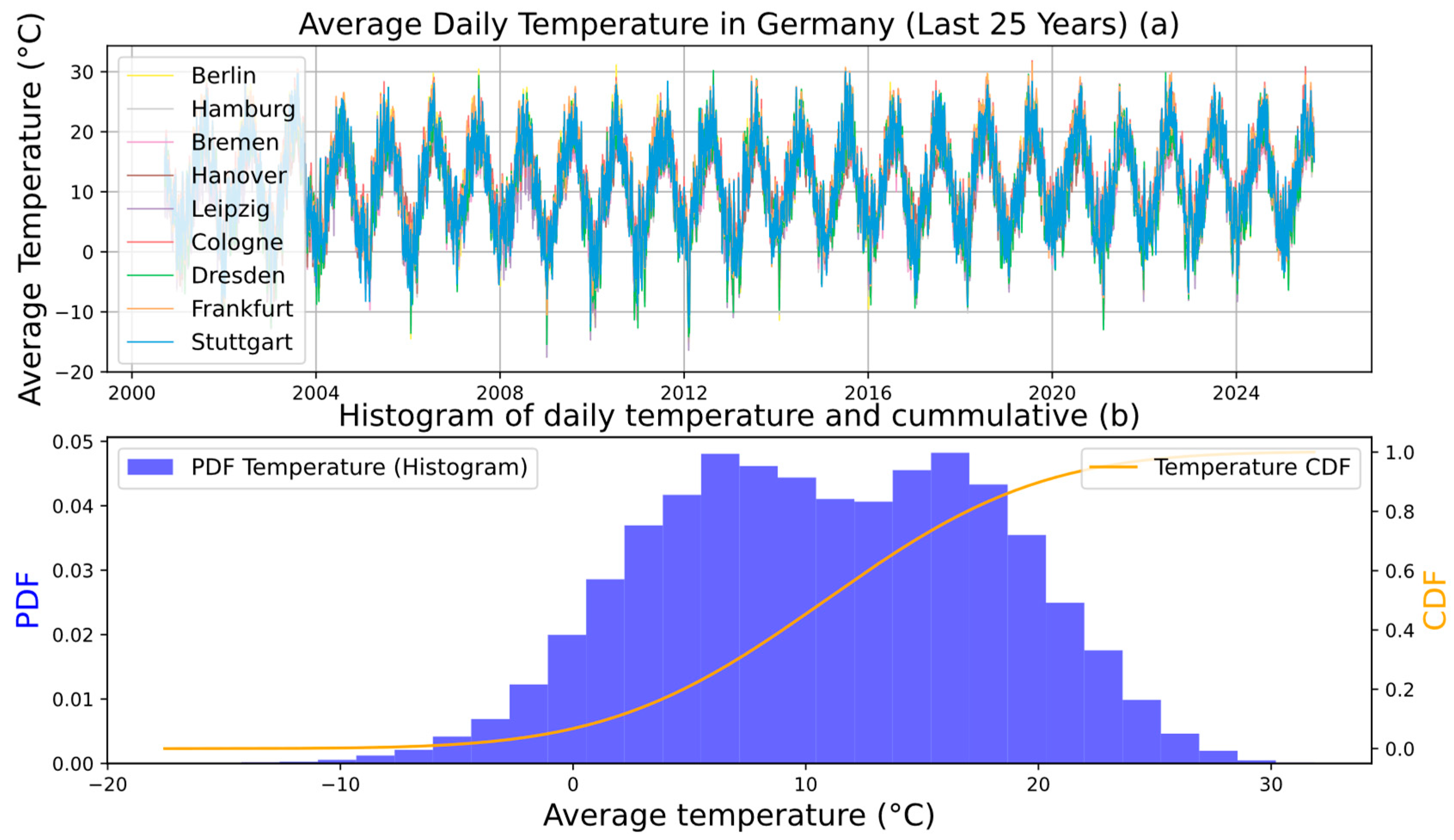
The locomotive is designed to run in all of Germany. To consider the climatic conditions of Germany, we have extracted meteorological data for the last 25 years from Meteostats [18] for the nine main cities of Germany (Bremen, Berlin, Cologne, Dresden, Frankfurt, Hamburg, Hanover, Leipzig and Stuttgart). The PDF and CDF are represented in Figure 9. As the law seems not to follow a standard probability density function, we have decided not to fit any classic probability laws, and instead use the histogram as calculated.

Concerning the SOH of the components, we will age the ESU and the FC together. We will consider two states, as the aging is considered linear over time—the BoL (Beginning of Life) and the EoL (End of Life). For the battery, the aging is simple; the internal resistance is increased up to twice the BOL value at the EOL. The capacity is reduced by 20% at the EOL to reach 80% of the BOL capacity. The FC is more complex; the polar curve is updated and so is the efficiency, but the auxiliary consumption cannot be shared for confidentiality reasons. As the components age linearly, the BOL and EOL will have the same occurrence probability of 50% each.

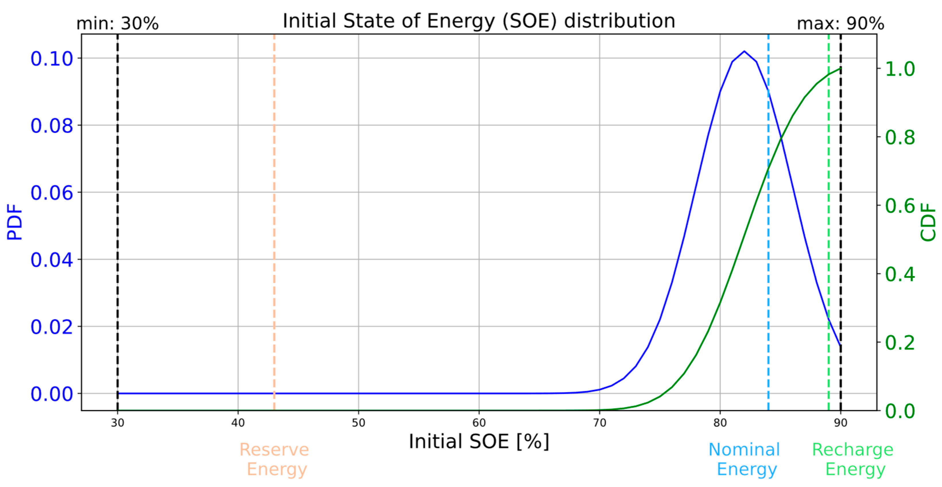
The last two factors in the scenario are related to the initialization of the simulation. These factors account for the fact that, prior to the current mission, any number of situations could have occurred. The first factor is the initial state of energy at the beginning of the mission. Although the EPMS is designed to regulate the state of energy close to the nominal value (84%), modeling a normal distribution centered at 84% would result in a probability that is too high, of nearly 90%, which is the maximum allowed energy. Moreover, the likelihood of ending a mission with an undercharged battery is higher than of ending it with an overcharged one. Therefore, the mean value was set at 82%. A standard deviation of 5% was chosen to reflect the variability in the final charge level after each mission. Finally, the normal distribution is truncated to remain within the operational range of the battery, which is between 30% and 90%. The corresponding probability density function is shown in Figure 10.

The last parameter is the initialization of the energy management law. As the law averages the power demand on the former moments, the past may have an impact on the way of working of the EPMS, mainly during the first minutes. As the missions are not predictable, the initialization follows a uniform law between the minimal possible power and maximum possible power.

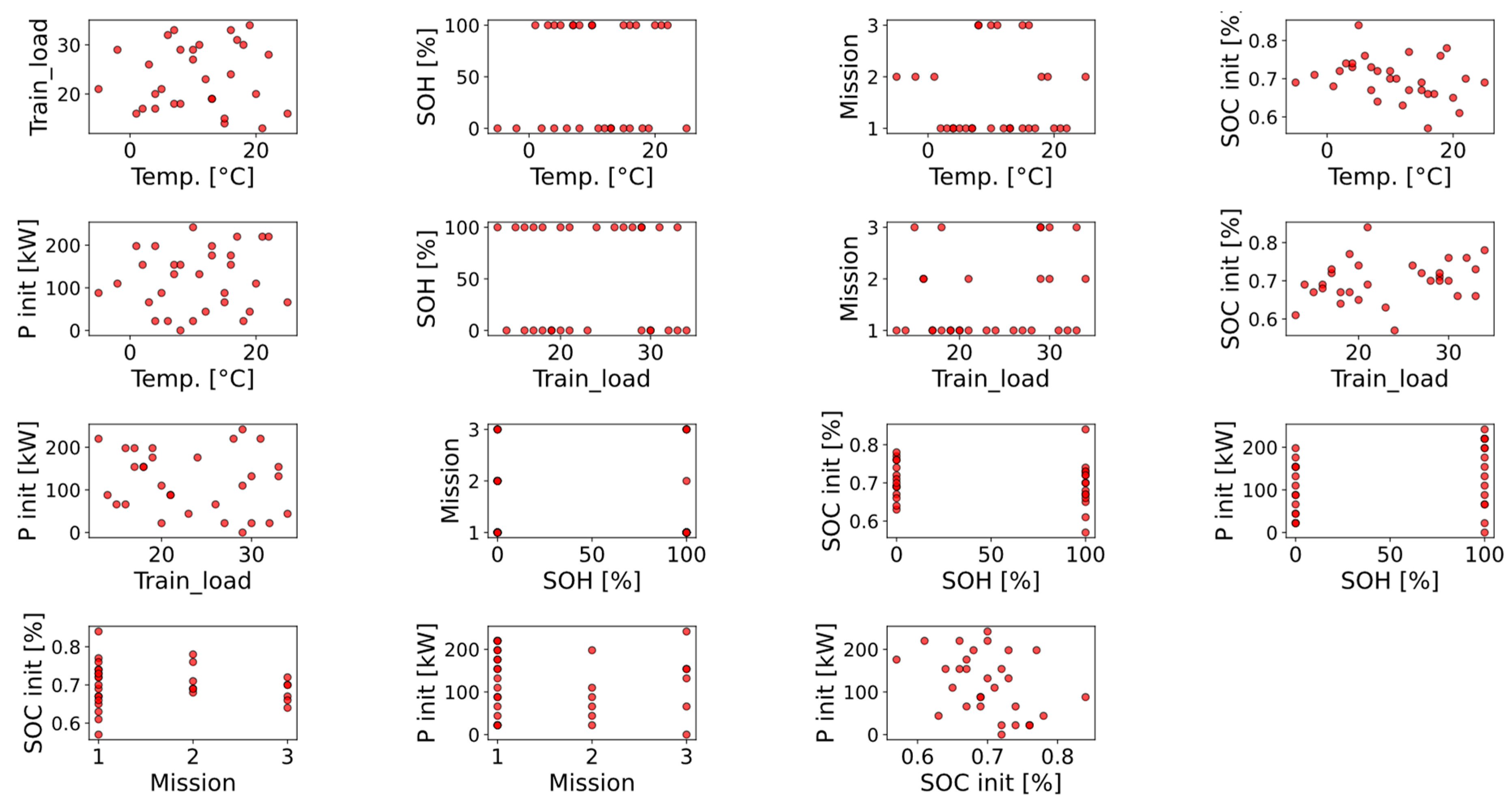
Finally, the 30 scenarios defined are represented in Figure 11. We can see that the points seem spread over each dimension, but the small number of points leaves huge empty areas.

In Figure 11, the first subgraph (row 1, column 1) shows the train load and temperature across 30 scenarios. Despite the limited number of data points, we can observe a good distribution across both scenario conditions. In the 13th subgraph (row 4, column 1), the scenario conditions are illustrated across three missions with their corresponding initial state of charge (SOC). Since the first mission is more likely to occur, we ensure the broader coverage of initial SOC values for this mission. In contrast, missions 2 and 3 focus more specifically on the most probable initial SOC values.

3.3. Optimal Parameter Combination

In this part we will define the objective function to be optimized and constrained. The number of configurations simulated is limited (100 to start). To minimize the objective function over the full EPMS configuration space, we need to be able to interpolate/extrapolate between the known configurations. A surrogate model will be trained in order to predict the missing configuration to ensure optimality throughout the whole EPMS parameter space. Finally, the method used to find the minimum objective function will be detailed.

3.3.1. Objective Function

The best EPMS will minimize four criteria, with the following order of priority:

-

The number of starts and stops for the FC;

-

The change rate of the FC;

-

The battery operates outside the nominal energy range;

-

The TCO of the mission (hydrogen cost and FC ageing cost).

The FC is designed with a maximum number of starts and stops before FC overhaul. To increase the lifetime of the FC, reducing the number of starts and stops per hour is crucial. The associated objective function is defined in Equation (17).

$${\mathrm{J}}_{\mathrm{F}\mathrm{C} \mathrm{s}\mathrm{t}\mathrm{o}\mathrm{p}\mathrm{s}}={\displaystyle \frac{nb stops}{T_{mission}}}$$

(17)

where ${\mathrm{J}}_{\mathrm{F}\mathrm{C} \mathrm{s}\mathrm{t}\mathrm{o}\mathrm{p}\mathrm{s}}$ is the objective function linked to the stop of the FC. $nb stops$ is the number of stops of the FC during the mission.

The locomotive hybrid system has been designed to be an RE. In order to respect this design, the FC power setpoint should not change quickly. On the contrary, the variation shall meet the requirements, but slowly. Besides this reference [19], has demonstrated that fast variations in the power of the FC are damaging. However, the data concerning our FC are unknown. We next check the amount of variation, and try to reduce it with Equation (18).

$${\mathrm{J}}_{F{C}_{change rate}}=\underset{0}{\overset{T_{mission}}{\int }}{\left({\displaystyle \frac{d{P}_{FC}}{dt}}\right)}^{2}dt$$

(18)

where ${\mathrm{J}}_{F{C}_{change rate}}$ is the objective function linked to the change rate of the FC.

The battery shall operate most frequently in the nominal energy area. The objective function will measure the energy needed outside the nominal energy area, and it is represented in Equations (19)–(21).

$${\mathrm{J}}_{ESU}={\mathrm{J}}_{ES{U}_{low}}+J_{ES{U}_{high}}$$

(19)

$${\mathrm{J}}_{ES{U}_{low}}=\underset{0}{\overset{T_{mission}}{\int }}\max \left(0, E_{mission}-\left(E_{ES{U}_0}+{\int }_0^t{P}_{ESU}\left(T\right)dT\right)\right)dt$$

(20)

$${\mathrm{J}}_{ES{U}_{high}}=-\underset{0}{\overset{T_{mission}}{\int }}\min \left(0, E_{recharge }-\left(E_{ES{U}_0}+{\int }_0^t{P}_{ESU}\left(T\right)dT\right)\right)dt$$

(21)

where ${\mathrm{J}}_{ESU}$ is the objective function linked to the energy level of the battery. ${\mathrm{J}}_{ES{U}_{low}}$ and ${\mathrm{J}}_{ES{U}_{high}}$ are, respectively, the objective functions covering the battery used in the low-energy area and in the high-energy area. $E_{ES{U}_0}$ is the initial level of energy in the battery used for the mission. $E_{mission}$ represents the lower threshold of energy of the nominal area and $E_{recharge}$ the upper threshold of the nominal area.

The last criterion is linked to the cost of the mission. It is comprised of two parts the cost of hydrogen in $ and the impact of the operating point of the FC on its ageing also in $. Concerning the ageing law used, we based the study on [16], where the authors studied the state of the art of the ageing laws for the FC and extracted an average value. The TCO objective function is defined by Equation (22).

$$J_{TCO}=\underset{0}{\overset{T_{mission}}{\int }}\dot{m_{H_2}}\left(t\right) dt.C_{H2}\left[USD/kg\right]+C_{FC}\left[USD\right].\underset{0}{\overset{T_{mission}}{\int }}{\displaystyle \frac{dmg\left(P_{FC}\right)\left[\mu V/h\right]}{\Delta V_{BOL-EOL}\left[\mu V\right]}}dt$$

(22)

where $J_{TCO}$ is the objective function linked to the TCO of the mission. $m_{H_2}$ is the H₂ mass flow. $C_{H2}$ and $C_{FC}$ are, respectively, the price of H₂ and of the FC system. $dmg\left(P_{FC}\right)$ is the damage function extracted from [16], it links the damage of the FC with the operating setpoint of the FC. $\Delta V_{BOL-EOL}$ is the voltage drop between the FC in BOL and EOL.

For each EPMS parameter combination, the objective functions defined previously will be evaluated over all the scenarios to ensure the robustness of the parametrization. To evaluate the objective function over all the scenarios, the expected value will be used for each objective function, represented by Equation (23).

$$\begin{gathered} J_{parameter, j}={\displaystyle \frac{1}{\sum _{i \in scenario}P\left(mission=i\right)}} .\sum _{i \in scenario}{J}_{mission, j }\left(i\right).P\left(mission=i\right) \\ for j \in objective functions \end{gathered}$$

(23)

where $J_{parameter, j}$ is the expected value of the jth objective function for a parameter combination over all the scenarios. $J_{mission, j }\left(i\right)$ is the jth objective function on the ith scenario. $P\left(mission=i\right)$ is the occurrence probability of the ith mission.

3.3.2. Surrogate Model

In [20,21], the authors used RSM trained on a set of simulations to estimate the optimal hybrid sizing. The idea is to train surrogate models (such as RSM or ML models) to extrapolate the performance of configurations that were not simulated, based on those that were.

Each surrogate model is trained separately for each objective function, in order to predict its value as accurately as possible. Since most RSM or ML algorithms typically produce a single output, we will describe the method for a generic objective function. The same approach is then applied to all objective functions. The parameters and results will be provided individually for each one.

The method of generating the surrogate model follows the ensuing steps:

• The dataset is split between training set and testing set (80%/20% of EPMS configurations);
• The model is trained on the training set until the hyperparameters of the model give good accuracy;
• The model is tested on the testing set to evaluate the capacity of the model to generalize on unseen configurations and avoid overfitting;
• Steps 2 to 3 are repeated for each objective function.

After testing several ML algorithms, the best results were obtained using a deep dense neural network (NN). The NN was implemented using the TensorFlow library [22] and the Scikit-learn library [23].

The principles of NN and their training are detailed in [24,25]. Here, we focus only on the specific aspects of our implementation. The neural network architecture used for all objective functions is the same, as is summarized in Figure 12, and the hyperparameters are also the same and are summarized in

Table 3. Hyperparameters of the neural network used.

Hyperparameter	Neural Network
Layer number	2
NL1/NL2	64/32
Activation function	ReLu/ReLu
Drop-out	0.2/0.2

.

To enhance the predictive capabilities of the NN, multiple models were trained sequentially for each objective function, following a structure similar to the XGBoost approach used for decision trees. This architecture, illustrated in Figure 13, will be referred to as the Neural Network Gradient Boost Model.

The first stage is trained to predict the target output, using the Mean Squared Error (MSE) as the loss function, as shown in Equation (24). Subsequent stages are trained on the residuals—the difference between the predictions of the previous stages and the actual output. Each additional stage incrementally improves the overall predictive performance of the model. These stages also use the MSE loss function, as indicated in Equation (25).

Training was conducted using the Adam optimizer over 400 epochs for each neural network stage.

$$L_1\left(\theta \right)={\displaystyle \frac{1}{N}} \sum _{i=1}^N{\left|\left|{f_1}_{\theta }\left(x_i\right)-y_i\right|\right|}^2$$

(24)

$$L_j\left(\theta \right)={\displaystyle \frac{1}{N}} \sum _{i=1}^N{||{f_j}_{\theta }\left(x_i\right)-{(y}_i-\sum _{k=1}^{j-1}{f_k}_{\theta }\left(x_i\right)) ||}^2 for j>1$$

(25)

where $L_j\left(\theta \right)$ is the MSE of the NN with j stages for the parameters $\theta$ and N is the number of data points in the dataset. $x_i \mathrm{a}\mathrm{n}\mathrm{d} y_i$ represent the input and output values of the i-th data point. Specifically, $x_i$ corresponds to the EPMS parameters (T_short, T_medium, T_long, α_medium), and $y_i$ is the output of the objective function J_parameter,j. Finally, ${f_j}_{\theta }$ denotes the model’s prediction of the jth NN stage for a given input.

The final output of the NN Gradient Boost model is the sum of the outputs from all stages, as defined in Equation (26):

$${\widehat{y}}_{final}= \sum _{j=1}^{N_{stages}}{f_j}_{\theta }\left(x_i\right)$$

(26)

where ${\widehat{y}}_{final}$ is the final output of the NN gradient boosting model. $N_{stages}$ is the number of neural network stages in the model (listed in

Table 4. Hyperparameters for NN gradient boosting.

Hyperparameter	J Stop FC	J Rate FC	J ESU	J TCO
NN stage number	3	3	4	1

for each objective function).

Finally, the performance of each NN Gradient Boost model for each objective function is presented in

Table 5. Performances of every model of each objective function.

Results	J Stop FC	J Rate FC	J ESU	J TCO
MSE train dataset	0.005	0.06	0.005	0.04
MSE test dataset	0.05	0.24	0.06	0.08
R2 train dataset	0.99	0.94	0.99	0.96
R2 test dataset	0.97	0.8	0.96	0.85

, using two evaluation metrics: Mean Squared Error (MSE) and the coefficient of determination (R²). These metrics were computed on both the training and testing subsets of the dataset. The data are normalized using the z-score method, resulting in a mean of 0 and a standard deviation of 1. Consequently, 99.7% of the values fall within the range of −3 to 3. Under this normalization, a MSE below 0.1 is considered very low, indicating extremely high model accuracy. An MSE below 0.5 is still regarded as low, reflecting good accuracy. In our case, the MSE values for both the training and testing datasets are below 0.1 for three of the objective functions. The only exception is the J rate FC, which has an MSE above 0.1 on the testing dataset, but it is still below 0.5, indicating good accuracy nonetheless.

Figure 14 shows all configurations simulated (over 100). The configurations are separated into training (blue) and testing (orange) sets, with both their original (light) and predicted (dark) values for each objective function.

3.3.3. Optimization

Since the optimization algorithm can only minimize a scalar function, all objective functions are combined into a single final objective function, as defined in Equation (27).

$$J_{parameter}={\beta }_{FC stops} . J_{FC stops}+{\beta }_{FC rate} . J_{FC rate}+{\beta }_{ESU}. J_{ESU}+{{\beta }_{TCO} J}_{TCO}$$

(27)

where $J_{parameter}$ is the final objective function for an EPMS parameter combination. $\beta$ is the coefficient used to resize all the objective functions and to give priority following the order defined in Section 3.3.1. The determination of the coefficients starts with the calculation of the standard deviation of each objective sub-function on the set. Then, we want to resize each sub-function to impose the standard deviation. Indeed, when optimizing, the target is to reduce the amplitude of the objective function. The higher the standard deviation, the sooner the optimization will search in this direction, and the higher the gain. Following this logic, the ${\beta }_{FC stops}$ has been resized to have a standard deviation of 40 on the FC stop objective function, which is the priority. The coefficient values and the standard deviation of their resized objective subfunction (${\sigma }_J)$ are provided in

Table 6. Beta coefficients of the final objective function.

Coefficient	${\mathit{\beta }}_{\mathit{F}\mathit{C} \mathit{s}\mathit{t}\mathit{o}\mathit{p}\mathit{s}} \left[\mathbf{h}\right]$	${\mathit{\beta }}_{\mathit{F}\mathit{C} \mathit{r}\mathit{a}\mathit{t}\mathit{e}} [{\mathbf{s}}^2/{\mathbf{k}\mathbf{W}}^2]$	${\mathit{\beta }}_{\mathit{E}\mathit{S}\mathit{U}} [\mathbf{k}{\mathbf{W}}^{-1}.{\mathbf{h}}^{-2}]$	${\mathit{\beta }}_{\mathit{T}\mathit{C}\mathit{O}} \left[{\mathbf{E}\mathbf{U}\mathbf{R}}^{-1}\right]$
coefficient	1000	2.7 × 10−4	7 × 10−2	1.1
${\sigma }_J$	40	10	5	5

.

The method to find the optimum is defined by the following steps:

-

Train the surrogate model;

-

Run the minimum research algorithm on the $\widehat{J_{parameter}}$, which is composed of the sum of the surrogate models with their beta coefficients, to find an optimal configuration;

-

Simulate the optimal configuration on all the scenarios and compute the $J_{parameter}$;

-

If the estimation and the result of the simulation match, then the optimum has been found. Otherwise, repeat the first steps, including the new combination simulated.

The differential evolution (DE) metaheuristic, as defined in [26], was used to search the minimum of the problem. One of the main advantages of DE is that it does not make any assumptions about the nature of the problem, making it suitable for exploring large and complex search spaces like ours. However, a limitation of DE is that it cannot guarantee that the solution found is the global optimum.

DE begins by initializing a population of candidate solutions. It evaluates the fitness of each individual using the final objective function. The best-performing individuals are retained, while the others undergo mutation through random modifications. These mutated individuals are then re-evaluated to form a new generation. The optimization process continues until a convergence criterion is met. The parameters used for the DE optimization are summarized in

Table 7. DE parameters.

Strategy	MaxIter	Popsize	Tolerance	Mutation	Recombination
best1bin	1000	15	0.01	(0.5, 1)	0.7

.

The optimum found by the DE algorithm is summarized in

Table 8. EPMS parameters for the reference and the optimal solution.

Tshort/Tmedium/Tlong	αshort/medium	Jparameter (Model)	Jparameter (Simulation)
600/1800/3600	0.5/0.5	-	937
545/1000/3900	0.63/0.37	888	899

. The best EPMS configuration is presented along with the predicted values from the models. Subsequently, simulations were performed across the entire set of scenarios, and the objective functions were evaluated based on the simulation results.

Figure 14 illustrates the results for each criterion, comparing the reference solution, the predicted optimum, and the simulated optimum. The predictions closely match the actual values, with an error margin of only 1.2%. The optimal EPMS parameter combination appears similar to the reference solution; however, these slight adjustments lead to notable improvements—the average number of start–stop events is reduced by 6%, and power variations are decreased by 15%. Additionally, battery usage outside the nominal range is minimized by 5%. All these improvements are achieved without any impact on the TCO.

This study highlights the following conclusions. For our application, the number of start–stop events and the usage of the ESU within its nominal range exhibit similar trends. Likewise, the TCO and FC power variations also follow similar patterns. However, the first two criteria show opposite tendencies compared to the latter two, making it challenging to optimize all objectives simultaneously. The prioritization order of the objective functions significantly influences the optimal solution.

3.3.4. Validation

The validation dataset is defined by the specification of the locomotive. The scenario validation dataset is composed of four missions. These missions are concatenations of simpler missions. The details of the four missions are given in Appendix B.

The reference solution and the optimal solution were simulated on the validation scenarios. The comparison of the optimal solution to the reference solution for all four validation scenarios is given in

Table 9. Comparison of the optimal solution to the reference solution in the validation scenarios.

Scenario	J Stop FC	J FC Rate	J ESU	J TCO	J Parameter
Validation n°1	0	+4%	−1%	−1%	−1%
Validation n°2	0	−1%	−1%	−1%	−1%
Validation n°3	0	+3%	−4%	0	−4%
Validation n°4	0	−9%	−2%	−6%	−2%

.

Globally, the optimum reduces all the objective functions. On average, the global objective function (J_parameter) is reduced by 2% for all validation scenarios. However, we can observe an increase in the FC power variations on validation scenarios 1 and 3. These results still demonstrate the validation of the methodology as a robust optimization.

4. Discussion

During the implementation of the proposed methodology, two primary challenges were encountered.

First, despite efforts to comprehensively define the scenario conditions, a key variation related to the stochastic nature of the shunting cycles was initially overlooked. All cycles followed an identical pattern, and during the optimization of FC power variations, the configurations that aligned precisely with this pattern yielded the best results. Consequently, a reduced weight was assigned to FC power variation in the final objective function to mitigate this bias.

Second, during model training, it was observed that conventional hyperparameter optimization techniques were ineffective. Specifically, subdividing the training dataset to perform hyperparameter tuning led to significantly degraded performance. In contrast, utilizing the full training dataset produced highly accurate results, as demonstrated in the study. This suggests that the initial dataset should have comprised 150 configurations (i.e., 4500 simulations) rather than 100 configurations (3000 simulations). This insight provides a valuable direction for future investigations.

The objective function consists of four components. Analysis revealed that these components exhibit paired behavior; that is, the number of FC stops and the nominal operating range of the ESU tended to vary together, while FC power variation and TCO also showed a correlated behavior, albeit in opposition to the first pair. The link between the ESU range and the FC shutdowns is straightforward when considering the implemented state law. Specifically, when the battery operates at a high energy level, an FC shutdown is triggered. Therefore, the longer the battery remains at a high energy level, the greater the probability of requesting an FC shutdown. Although the ESU objective function also considers low energy levels, these are rarely reached due to the appropriate sizing of the hybrid traction drive. The final trade-off was primarily between minimizing the number of FC start–stop events and reducing FC power variation.

The predictive performance of the machine learning models was notably high, with prediction errors on the global objective function frequently below 1%.

However, the observed savings in the validation scenarios were limited. This is attributed to the optimization being focused on minimizing FC start-stop events, whereas the validation missions did not trigger any such events.

5. Conclusions

The optimal solution identified through the proposed methodology ensures the robustness of the EPMS parameter configuration across a wide range of scenario conditions. Although the savings may appear modest compared to the reference solution, it is important to note that the EPMS range extender control strategy was designed with these parameters in mind. Ensuring the robustness of this control law while simultaneously enhancing the longevity of both the fuel cell and the battery represents a significant achievement. The average savings over the 30 scenarios have been estimated at between EUR 800,000 and EUR 1 million for a locomotive over a 30-year period, primarily due to the reduction in start–stop cycles. These savings are achieved through an automated method that completes its calculations in under one day. The results prove that the methodology can be defined as a framework to tune different EPMS laws over a large range of operations.

The next step of the study will be the implementation of the optimal parameter combination found during the study. The correlation of the expected results with the real measurements will be part of the validation of the method.