Abstract
The Pyrenean capercaillie (Tetrao urogallus aquitanicus) is a forest obligate grouse that has experienced a marked population decline in recent decades owing to the lack of optimal habitats. However, the effect of forest structure on potential predators and habitat competitors has not been well-studied. We conducted a camera-trapping study at three conservation areas in Huesca province (northeastern Spain), which were classified as ‘optimal’, ‘favorable’, and ‘unfavorable’ based on habitat suitability for the capercaillie. This study was conducted for 3417 days at a total of 130 camera locations in autumn–winter and spring–summer, capturing 8757 valid photos. In total, 36 different species were recorded. The most frequently detected species were Southern chamois (Rupicapra pyrenaica pyrenaica; 32.6%), roe deer (Capreolus capreolus; 18%), wild boar (Sus scrofa; 9.6%), red squirrel (Sciurus vulgaris; 6.1%), mustelids (5.6%), and red fox (Vulpes vulpes; 4.8%). Capercaillies were photographed in the optimal and favorable habitat areas. Nest predators, such as mustelids and red fox, were more frequently detected in the favorable area during autumn–winter and in the optimal area in spring–summer, while corvids were more frequently detected in the unfavorable habitat area during both periods. No clear pattern was found for wild boar (nest predator and habitat competitor) or cervids (competitors). As capercaillie coexist with a wide range of predators and competitors, and habitat structure may not always explain species relative abundance, factors such as disturbance and food resources should be also taken into account when aiming to develop targeted management for the benefit of the capercaillie.
1. Introduction
The Pyrenean capercaillie (Tetrao urogallus aquitanicus Ingram, 1915), is an endangered bird that lives in alpine habitats of the Pyrenees, with populations in Andorra, France, and Spain [1], and is closely related to the Cantabrian capercaillie (T. urogallus cantabricus Castroviejo, 1967), which is distributed in northwestern Spain [2]. Like other members of the grouse family (Tetraonidae), the Pyrenean capercaillie (hereafter, PC), is a forest obligate species. In Spain, its occurrence is associated with coniferous forest (Scots pine Pinus sylvestris and mountain pine Pinus uncinata) and shrubs that provide shelter and food, including bilberry (Vaccinium myrtillus), alpenrose (Rhododendron ferrugineum) bearberry (Arctostaphylos uva-ursii), and common juniper (Junniperus communis) [3,4].
In Spain, the PC population has experienced a marked decline in recent decades. Among the different factors explaining this trend, habitat loss and fragmentation are considered the most important [4], though, as described for other subspecies, other factors may influence their population trends, such as climate change [5], human disturbances [6], and predators [5,7]. Available research shows that the most important PC predators are pine marten (Martes martes Linnaeus, 1758), red fox (Vulpes vulpes Linnaeus, 1758), golden eagle (Aquila chrysaetos Linnaeus, 1758), and goshawk (Accipiter gentilis Linnaeus, 1758) [8]. Moreover, the effects of ungulates in capercaillie habitats should also be taken into account; for example, wild boar (Sus scrofa Linnaeus, 1758) may prey on capercaillie nests (their eggs are laid on the ground, [9]), and medium-high densities of cervids can overgraze ground vegetation crucial for PC survival [10,11].
In recent years, studies have addressed the occurrence and abundance of predators in areas where the PC still exists [12,13,14], but there is a lack of knowledge about how forest structure influences the abundance of PC predators and habitat competitors. For other capercaillie populations, it is accepted that diverse and non-fragmented habitats may help to reduce predation risk at different life stages [15,16,17].
According to the Spanish national strategy to recover both the Pyrenean and Cantabrian capercaillie, at the moment, the main priority is habitat conservation. However, predator and ungulate removal are also considered when aiming to increase the observed poor breeding success, which is one of the factors triggering the decline in certain contexts [18]. A better understanding of the diversity and abundance of predators and competitors in different habitat contexts where capercaillie is currently present (or became extinct recently) could help to develop tailored management to benefit this endangered species.
In this study, we aimed to evaluate the abundance of predators and competitors of the PC in protected areas for the conservation of the species in the region of Aragón (north-eastern Spain), comparing areas with different habitat characteristics. Our information could inform the decisions of policy makers in the current scenario in which recovery efforts are being carried out to change the fate of this iconic species.
2. Materials and Methods
2.1. Study Area
This study was conducted in the municipality of Bielsa (Huesca province, Aragón, Spain, Figure 1), where the PC has been historically distributed, and as part of a recovery project following regional management capercaillie regulations to benefit the species [19]. In Bielsa, there are five declared protection areas for PC conservation (Figure 1). These areas are known to contain lekking sites (in Spanish called ‘cantaderos’) and are part of six Natura 2000 sites (ES0000016, ES0000279, ES0000280, ES2410019, ES2410052, and ES410053). Two of these critical areas are within the influenced area of the ‘Ordesa y Monte Perdido National Park’, which holds the highest level of nature protection in Spain.
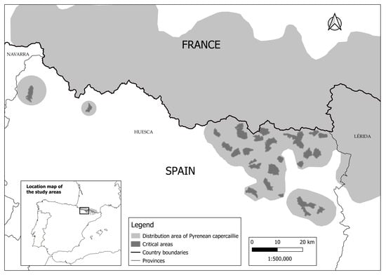
Figure 1.
Distribution range of the Pyrenean capercaillie in Aragón and neighboring regions of Spain and France, showing the three study areas within the critical areas for the conservation of the species.
In this part of the Pyrenees, the PC lives in mature coniferous forest dominated by mountain pine, in subalpine habitats with Scots pine and, to a lesser extent, European larch (Larix europaea) and spruce (Picea abies), in combination with shrubs that provide shelter, food, nesting substrate, and chick-rearing habitats [4].
One of the most commonly used variables to describe habitat favorability for capercaillie is the percentage of tree canopy cover (TCC). A TCC of 50% is considered optimal across its range, including in Scandinavian and Alpine coniferous forests [20,21], as well as in the Pyrenees [3]. In addition to TCC, the height, fruiting capacity, and ground cover percentage of shrubs are also important factors in determining habitat suitability [21,22]. Generally speaking, a higher percentage of shrub cover increases habitat suitability, as it provides a greater surface area for breeding and protection against predators. In the Pyrenees, a shrub cover between 75 and 90% is considered optimal, between 25 and 75% favorable, and below 25% unfavorable [23].
This study was conducted in three conservation areas in which we aimed to address whether PC was present, identify conservation problems, and analyze the habitat characteristics. Considering the historical PC lekking sites in each area, provided by the regional wildlife service, a plot of approximately 1.12 km2 around the lekking sites was selected for monitoring, with the lower altitude being 1500 and the upper limit marked by the forest (up to 2250 m).
We analyzed habitat suitability for PC in the study areas using maps produced by GIS tools and field-collected data. As a reference, we used the optimal, favorable, and unfavorable percentage values for TCC and shrub species cover described earlier.
To determine the favorability of forest canopy cover in each study area, we used the high-resolution raster layer of TCC from Copernicus 2018 (10-m resolution) (High-Resolution Layer Tree Cover Density, www.copernicus.eu (accessed on 11 October 2023). For understory cover suitability, we used field-collected data and shrubland cover data from SIOSE (Land Occupation Information System of Spain, www.siose.es, accessed on 11 October 2023). To assess the percentage of forest area dominated by broadleaf species, we utilized the High-Resolution Layer Dominant Leaf Type from Copernicus 2018. The tree species composition in each area was obtained from the Spanish Forest Map [24].
2.1.1. Area 1, ‘Optimal’
This area (4.6 km2) provided favorable tree canopy conditions, with a TCC of 50.92%, but the understory cover was suboptimal. The presence of broadleaf species was low (2.66%), with beech (Fagus sylvatica) occurring in 10–20% of the lower Scots pine forest, but absent in the higher mountain pine areas. The south-facing orientation and limestone soils held juniper and bearberry, but bilberry was nearly absent and non-fruiting. In denser forest areas, the understory cover was low due to junipers’ shade intolerance, while open areas have up to 30% juniper cover. This site had the highest proportion of grassland (25%), and 15.09% of the area lacked tree cover, consisting of rocky terrain and forest clearings, which enhances PC habitat. The lekking site remained occupied, but only one male was detected in counts prior to the study.
2.1.2. Area 2, ‘Favorable’
This area (7.15 km2) offered the most favorable habitat conditions, with a TCC of 69.28% and areas with optimal understory cover. The forest was dominated by Scots pine at lower elevations, transitioning to mountain pine at higher elevations, with minimal broadleaf presence (0.34%), although rowan (Sorbus aucuparia) was found in certain north-facing sectors. Unlike the other sites, this area included both north and south-facing slopes, increasing shrub diversity. North-facing slopes had highly PC favorable rhododendron cover (80–90%) and frequent bilberry occurrence, while south-facing slopes had lower shrub cover (10–30%), mainly juniper and bearberry, with some areas lacking any understory cover. The presence of forest clearings, rocky zones, and well-covered grasslands (7.31% of the area without trees) increased habitat quality. This site supported the highest number of detected PC (three males) compared to nearby critical areas.
2.1.3. Area 3, ‘Unfavorable’
This area (7.9 km2) had the least favorable habitat conditions, with a high TCC (85.22%), creating a dense forest with minimal open spaces. The north-facing orientation supported silver fir (Abies alba) in varying proportions, from 80% dominance in some areas to 10–40% in mixed stands with mountain and Scots pine. Broadleaf species were scarce (2.13%), and the understory cover was dominated by rhododendron and bilberry, although most of the area lacked this vegetation. The absence of forest clearings and the low presence of grasses reduced the habitat suitability. No PCs have been detected in this area in the last 10–15 years (Figure 2).
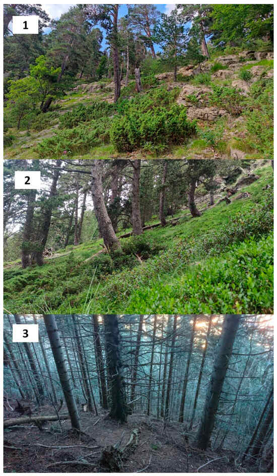
Figure 2.
The three areas in which the study was conducted; area 1 (optimal), with appropriate forest canopy cover (FCC), rocky ground, and patchy shrub vegetation; area 2 (favorable), with favorable FCC and abundant shrub vegetation; and area 3 (unfavorable), with non-favorable FCC and the absence of shrub vegetation.
2.2. Camera Trapping and Transects
As the majority of potential PC predator and competitor species are elusive (mesocarnivores and ungulates), camera trapping was used for monitoring. Each 1.12 km2 plot was divided into 200 × 200 m grids (28 plots of 0.04 km2), and one camera trap was located at approximately the center point of each grid (depending on access and camera availability). Minimum and maximum distances between the cameras were established to avoid overlapping (250–350 m), depending on the slope and habitat characteristics in each plot. With this network of cameras, we aimed to monitor the lower and upper limits in each area (Figure 3).
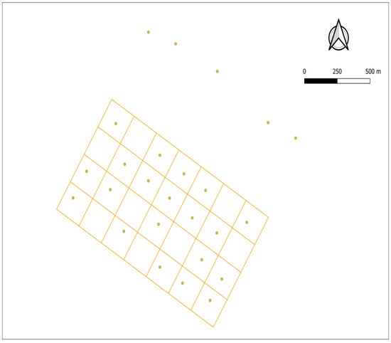
Figure 3.
Spatial arrangement of the camera traps in one of the study areas (showing in red the limits of the critical area), in which a total of 20 cameras were deployed in autumn–winter. In this area, 5 cameras were deployed outside the grid to monitor wildlife and possible human disturbances coming from a track.
The Browning Dark-Ops © camera trap model was used for the entire duration of the study, using a photo resolution of 12 megapixels and a trigger response of <1.2 s. We set the cameras to work 24 h/day, programmed with a medium-sensitivity sensor setting, to take 2 photos when triggered and with a time delay of 1 min between consecutive triggers. Based on previous studies conducted on similar species in the Pyrenees [25], and findings from other Iberian ecosystems [26], we aimed to achieve a minimum of 20 days of monitoring per camera trap; therefore, the cameras were deployed for periods of 25–35 days to increase the detectability of the target species.
All cameras were installed on trees, at an approximate height of 0.5–2.0 m off the ground, pointing to a bait, and avoiding orientations that could lead to photo overexposure. The locations were chosen considering accessibility, focusing on areas in close proximity of tracks and runs. To increase the detection probability of mammal species, baits (valerian extract and fish oil) were placed on a metal rod at about 0.5 m above the ground, set at 2–4 m from each camera [27].
We aimed to evaluate the occurrence and relative abundance of the target mammal species at the areas in two main periods. The first round was conducted in autumn–winter, using valerian extract [28], and the second round in spring–summer, using fish oil as bait. Owing to the limited number of cameras available (range of 19–25), it was not possible to monitor the areas simultaneously, though monitoring overlapped between areas in some cases because the cameras were retrieved and deployed in batches, and from November 2019, more cameras were available.
The starting and finishing dates for each area and period (autumn–winter and spring–summer) were as follows: area 1 (optimal), from 10 October to 11 November 2019 and from 13 April to 11 May 2020; area 2 (favorable), from 11 November to 3 December 2019 and from 23 July to 30 August 2020; area 3 (unfavorable), from 6 November to 8 December 2019 and from 29 May to 1 July 2020. The spring–summer period was longer owing to movement restrictions during the COVID-19 lockdown, which made it difficult to complete monitoring in a shorter period of time. Weather data was retrieved from an official weather station located in Bielsa (https://www.aragon.es/-/clima-/-datos-climatologicos#anchor2, accessed on 12 May 2025).
Together with camera trapping, we conducted two walked transects at the plots before and during camera deployment, selecting vantage points to observe potential PC predators that could be difficult to detect through camera trapping, such as raptors and corvids. During these transects, we collected signs of PC presence, mainly feces and feathers.
2.3. Data Analysis
During each period, every grid was monitored by a camera trap, using the same locations during both monitoring periods. Therefore, the unit of analysis was the camera in a given location. In each photo, the time (hour and minutes), species, and the total number of animals per species were recorded. The identification of individuals was not possible, with the exception of wild cats (Felis silvestris Schreber, 1775) and some ungulates whose antlers could be assigned to one individual. Considering the main predators and possible PC habitat competitors, we categorized the species photographed into seven groups for the analysis: cervids, corvids, mustelids, Southern chamois (Rupicapra pyrenaica pyrenaica Bonaparte, 1845), wild boar, rodents, and red fox (Appendix A).
Following the approach of Armenteros et al. [29], we explored different intervals (5, 10, 15, 20, and 30 min) to minimize the risk of using consecutive photos of the same individual or species group. We decided to use only photos of the same species separated by a minimum of 15 min (valid photos), which were considered independent detections. Owing to the differences in the number of days the cameras were deployed, we calculated in each camera location the number of valid photos per day, which was used as a relative abundance index (RAI) for each group of species.
All statistical analyses were performed with R version 4.4.2 [30], using tests with base R functions. The data from each period (autumn–winter and spring–summer) were loaded and processed separately to examine differences between periods. For each group of species, descriptive statistics of the RAI were calculated by area (mean, standard deviation, minimum, and maximum). The aggregate function in R was used to compute these statistics for each species across the three areas. As the data did not meet the assumptions of normality, non-parametric tests were used. To assess whether there were significant differences in the RAI between groups of species and areas, Kruskal–Wallis tests were performed, and Wilcoxon–Mann–Whitney tests were conducted to compare the relative abundances between the two periods for each group of species [31]. The p-values were expressed according to the method of Muff et al. [32].
3. Results
After checking the cameras and excluding those that malfunctioned, camera trapping was conducted over 3417 days across a total of 130 camera locations (26.3 days/camera trap), inclusive of the two rounds (Table 1). The total number of valid photos for the analysis was 8757, and 36 different species were recorded, including 18 mammals (including cattle and dogs) and 18 birds (Figure 4, see Appendix A). Pooling all photos from the three areas, the most photographed species were Southern chamois (32.6%), roe deer (Capreolus capreolus Linnaeus, 1758; 18%), wild boar (9.6%), red squirrel (Sciurus vulgaris Linnaeus, 1758; 6.1%), and red fox (4.8%). We had difficulties when distinguishing between stone (Martes foina Erxleben, 1777) and pine marten; therefore, these photographs were classified as ‘Martes foina/martes martes’, and afterward, merged into the category ‘mustelids’ (5.6%). It was possible to photograph PC in areas 1 and 2, although the number of photos was rather low (20). Taking all cameras from the two rounds, the most frequent detected groups were cervids (73.7%) and chamois (72.4%), while the less frequent were rodents (21.1%) and corvids (22.6%). When looking at the species diversity recorded in each area, out of 33 different wild species detected during the study, 69% were detected in area 1, 48% in area 2, and 45% in area 3.

Table 1.
The number of cameras, camera-trapping days, valid photos, and proportions of cameras in which the different groups of target species were detected per area and round (AW = autumn–winter, SS = spring–summer). For each area, the following weather data are given considering the months in which cameras were deployed: mean temperature (°C), mean maximum temperature (°C), mean minimum temperature (°C), and accumulated rainfall (mm).
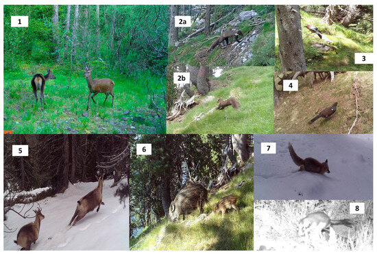
Figure 4.
Main group of species photographed at the study sites; (1) cervids, (2) mustelids (pine marten (2a), and unknown mustelid (2b)), (3) corvids (jay), (5) chamois, (6) wild boar, (7) red fox, and (8) rodent (dormouse). The Pyrenean capercaillie was also photographed but at a lower rate (4).
In autumn–winter, there were strong significant RAI differences among the areas for mustelids (H = 12.13, p = 0.002), chamois (H = 25.01, p < 0.001), and wild boar (H = 12.28, p = 0.002), with higher values of these groups recorded in area 2, and moderate evidence of corvids (H = 7.62, p = 0.022), for which higher values were reported in area 3. In this period, rodents had moderately higher RAI values in area 1 compared to the others (H = 6.92, p = 0.031).
In spring–summer, different patterns were found. In area 1, there were high RAI values for foxes (H = 10.42, p = 0.005), in area 2 for cervids (H = 10.04, p = 0.006), chamois (H = 10.70, p = 0.004), and wild boar (H = 6.74, p = 0.034), and a lower value in area 2 for corvids (H = 7.94, p = 0.018). When comparing the RAIs between the rounds, there were highly significant differences among the areas for mustelids (H = 1080, p < 0.001) and wild boar (H = 1171, p < 0.001; a higher RAI was reported in spring–summer). Moderate evidence was found for differences in the RAI for chamois (H = 2591, p = 0.015), while there was no evidence of differences for rodents (H = 1946.5, p = 0.371) (Table 2, Figure 5).
Table 2.
Kruskal–Wallis and Mann–Whitney U test results when comparing the relative abundance index (RAI) for the groups of species considering each round (AW = autumn–winter, SS = spring–summer) and the two rounds.
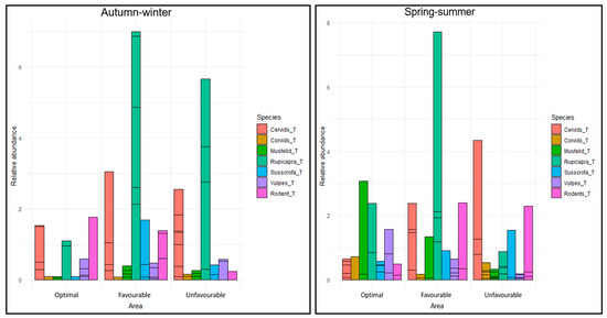
Figure 5.
Relative abundance index (number of valid photos per camera and days) per group of species, area, and period.
4. Discussion
To the best of our knowledge, this is the first study to evaluate the occurrence and relative abundance of predators and habitat competitors of the PC with camera trapping in the studied areas. Our results suggest that both habitat structure and the study period influenced the relative abundance of some groups of species, which could have management implications in the current context in which recovery programs are trying to reverse the negative PC trend.
Camera trapping allowed for the identification of the target species, together with other species occurring in the areas. Previous studies in similar mountainous areas have proved that camera trapping allows for the detection of a wide range of species [25,33], including small- and medium-sized carnivores in studies using artificial capercaillie nests [13]. The number of photos was overwhelmingly high for Southern chamois and roe deer, which is not surprising because these areas provide optimal habitats for them [34]. As the studied areas were just below upland areas, Southern chamois were frequently detected accessing the lower parts of the mountains after the first snow, which is a well-known behavior [35]. In contrast, corvids and rodents were less frequently detected groups of species. The former were mainly found in area 3, and the latter did not show a clear pattern, suggesting that camera trapping should be combined with other methodologies when aiming to obtain accurate data on these species.
All groups of species were detected in the three areas during the two rounds, and as expected, there were differences among the areas and rounds, with further differences observed between the rounds for some species. However, these results should be interpreted with caution owing to the different types of bait used and the monitoring periods, as we were unable to deploy cameras simultaneously in the three areas. The weather conditions (temperature and rainfall) between the periods was similar, with the exception of the spring–summer period in area 2, which was drier than the other monitoring areas. In any case, we chose periods covering the post-breeding season (autumn–winter) and the breeding season (spring–summer) for the majority of the species to compare possible differences between the periods. We did not test the effect of baiting on detection using camera traps without bait because we aimed to optimize the efforts, as previous research has proven that baiting increases detection probability for elusive species, such as mustelids [36].
The relative abundance of mustelids, which are key PC nest predators [37], was significantly higher in area 2 during autumn–winter, but this pattern changed in spring–summer, when the abundance was higher in area 1 and increased in all areas compared to the previous round. This is likely explained by their breeding season (which results in mustelids being more active), which also coincides with the PC breeding season. The difficulty in distinguishing between pine and stone martens limited a complete understanding of our results. Interestingly enough, we found a very similar pattern for foxes in round 2, with higher values compared to the autumn–winter period and a high abundance value in area 1 compared to the others. It may be that this area provided optimal hunting grounds and higher prey densities (mainly rodents). We cannot discard that these results reflect interactions between carnivores and prey, as rodents showed higher RAI values in spring–summer [38,39]. It is known that mustelids select forest in which grounds have cover vegetation, and stone martens can be also found within human settlements [40,41] while fox can be considered a generalist species and is virtually present in all types of habitats [42].
The abundance of corvids, mainly represented by the Eurasian jay (Garrulus glandarius Linnaeus, 1758), was significantly higher in area 3 for the two rounds and in area 2 for the spring–summer period, which points toward the idea that area 3 (which had the worst habitat conditions for the PC) offered optimal habitats for a known nest specialist predator [43], with a likely low impact for PC nests but still unknown.
Wild boar, which can be considered a habitat competitor for ground nesting birds [44] and also a predator [13], had higher abundance values in area 2 in autumn–winter, possibly associated with the lack of human disturbance during this period, when hunting battues were organized in the other areas [45]. In spring–summer, a higher abundance of wild boar was found in area 3, perhaps explained by a combination of lack of disturbance and a large proportion of bare ground available for rooting. Area 3 may have been used by deer as a protection area to avoid human disturbance, as there was a lack of ground vegetation. Although the wild boar abundance values were higher in spring–summer, likely due to the juvenile rearing period in the areas, the absence of a clear pattern could be attributed to its adaptability to different habitats, as it can be found in a wide range of habitats but at different densities [46]. With regard to cervids, we did not found a clear pattern (mainly represented by roe deer), as, during autumn–winter, no differences were found among the areas, and in spring–summer, higher abundances of cervids were observed in areas 2 and 3. Cervids are known to be distributed in a wide range of habitats within the region of Aragón, including the Pyrenees [34,42]; therefore, these differences could be related to factors other than habitat structure.
The case of the chamois is rather interesting because higher abundance values were observed during both rounds in area 2. As previously mentioned, this could be explained by the effect of snow, which compelled the animals to occupy the lower parts of the mountain in search of food, getting back to the summer habitats where grasslands were available [35].
Our study did not allow for an in-depth investigation of the interactions among different species, as we aimed to group the most important ones for comparison. As camera trapping did not target the PC, we could not assess whether predators and habitat competitors affected them; therefore, further studies are needed to address PC habitat selection and the possible influence of predators and habitat competitors, especially during the PC breeding season.
5. Conclusions
This camera-trapping study reveals that the PC coexist with a wide range of known predators and possible habitat competitors, regardless of the habitat structure. In areas 1 and 2, which had optimal and favorable habitats for the PC, predators and habitat competitors appeared and were frequently detected. Even when management is conducted to provide heterogeneous habitats to benefit PC, it may not significantly modify the relative abundances of predators and habitat competitors, mainly because the majority of species are able to adapt to different ecological contexts.
Secondly, as the relative abundance of mustelids was higher in spring–summer (coinciding with the PC breeding season), if these species were to be managed to reduce nest predation, removal efforts should be conducted before this period, as already conducted for capercaillies in other areas of the Pyrenees and the Cantabrian Mountains [18]. The same applies to foxes, for which a very similar pattern was found in spring–summer, which suggests that habitats with open patches and rocky grounds (as found in area 1) are used by these predators during the PC breeding season.
Lastly, the lack of clear patterns for wild boar and cervids suggests that the management recommendations for these species should be based not only on habitat structure, but also on other factors, such as food availability (including carrion for wild boar [14]). Together with camera -trapping, the collection of evidence of habitat competition, such as overgrazing by cervids and soil damage caused by wild boar rooting (as observed in some parts of area 3), could be a first step to assess whether these species may cause disturbance to the PC.
The combination of clear cutting and other habitat measures (as already conducted in some unfavorable areas by the Government of Aragón), ungulate control, and mustelid translocation to increase breeding success and recruitment (adapted to each context) [15,18] could change the fate of the PC in a current extinction scenario.
Author Contributions
Conceptualization, A.M. and C.S.-G.; methodology, A.M. and C.S.-G.; formal analysis, A.M., R.C. and I.N.; resources, C.S.-G.; data curation, A.M. and C.S.-G.; writing—original draft preparation, C.S.-G. and C.M.-C.; writing—review and editing, all authors; project administration, C.S.-G.; funding acquisition, C.S.-G. All authors have read and agreed to the published version of the manuscript.
Funding
This research was funded by Fondazione la Lomellina, the Regional Government of Aragón and core funds from Fundación Artemisan.
Institutional Review Board Statement
Not applicable. This research was an observation study; therefore, it did not involve handling animals. Access to critical areas was given by the regional government of Aragón.
Informed Consent Statement
Not applicable.
Data Availability Statement
Data is available upon reasonable request.
Acknowledgments
We are grateful to Fondazione la Lomellina and the Regional Government of Aragón for funding our capercaillie monitoring work, the Hunters’ Federation of Aragón (FAR), the wildlife wardens (APN), and the Regional Government for allowing access to the critical capercaillie conservation areas. We are indebted to the Hunters’ Association of Bielsa and its Town Council for their continuous support and commitment. Special thanks are given to M. Falabrino, M. Alcántara, R. López, J.L. Burrel, and R. Castillo-Contreras. Anonymous reviewers provided key comments to improve this manuscript.
Conflicts of Interest
The authors declare no conflicts of interest.
Abbreviations
The following abbreviations are used in this manuscript:
| PC | Pyrenean capercaillie |
Appendix A
The breakdown of species detected per area, showing the number of valid photos from the two rounds. The groups of species are also indicated. (*) Indicates inclusion in the mustelid group owing to a similar ecological functionality.
| Species | Group | Optimal | Favorable | Unfavorable | Total |
| Apodemus sylvaticus | Rodents | 22 | 9 | 85 | 116 |
| Bird (unknown) | 5 | 21 | 22 | 48 | |
| Bos taurus | 345 | 0 | 4 | 349 | |
| Canis lupus familiaris | 6 | 4 | 18 | 28 | |
| Capra aegragus hircus | 39 | 39 | |||
| Capreolus capreoulus | 124 | 588 | 867 | 1579 | |
| Cervid (unknown) | Cervids | 3 | 7 | 10 | |
| Cervus elaphus | Cervids | 60 | 76 | 87 | 223 |
| Columba palumbus | 21 | 15 | 36 | ||
| Corvus corax | Corvids | 19 | 19 | ||
| Cyanistes caeruleus | 1 | 1 | |||
| Dryocopus martius | 4 | 4 | 8 | ||
| Eliomys quercinus | Rodents | 187 | 5 | 192 | |
| Erithacus rubecula | 9 | 9 | |||
| Felis silvestris | 21 | 54 | 40 | 115 | |
| Fringilla coellebes | 2 | 2 | |||
| Garrulus glandarius | Corvids | 4 | 20 | 81 | 105 |
| Genetta genetta (*) | Mustelids | 2 | 2 | ||
| Homo sapiens | 32 | 37 | 69 | ||
| Lepus europaeus | 29 | 3 | 6 | 38 | |
| Marmota marmota | 5 | 5 | |||
| Martes foina/Martes martes | Mustelids | 266 | 129 | 67 | 462 |
| Medium size carnivore (unknown) | 1 | 13 | 3 | 17 | |
| Meles meles | Mustelids | 2 | 68 | 15 | 85 |
| Mustelid (unknown) | Mustelids | 1 | 7 | 25 | 33 |
| Ovis orientalis aries | 9 | 9 | |||
| Perdix perdix hispaniensis | 3 | 3 | |||
| Phylloscopus collybita | 2 | 2 | |||
| Picus viridis | 6 | 6 | |||
| Rodent (unknown) | Rodents | 80 | 105 | 59 | 244 |
| Rupicara rupicapra | Chamois | 261 | 1878 | 721 | 2860 |
| Sciurus vulgaris | 99 | 225 | 215 | 539 | |
| Scolopax rusticola | 2 | 2 | |||
| Sus scrofa | Wild boar | 74 | 270 | 499 | 843 |
| Tetrao urogallus | 8 | 12 | 20 | ||
| Turdus iliacus | 3 | 3 | |||
| Turdus merula | 2 | 11 | 29 | 42 | |
| Turdus philomelos | 4 | 64 | 27 | 95 | |
| Turdus pilaris | 8 | 8 | |||
| Turdus torquatus | 2 | 42 | 44 | ||
| Turdus viscivorus | 2 | 2 | |||
| Ungulate (unknown) | 6 | 3 | 14 | 23 | |
| Vulpes vulpes | Red foxes | 173 | 148 | 101 | 422 |
References
- Ménoni, E.; Leclercq, B. Le Grand Tétras; Biotope Éditions: Mèze, France, 2020; ISBN 9782366622133. [Google Scholar]
- Escoda, L.; Piqué, J.; Paule, L.; Foulché, K.; Menoni, E.; Castresana, J. Genomic analysis of geographical structure and diversity in the capercaillie (Tetrao urogallus). Conserv. Genet. 2023, 25, 277–290. [Google Scholar] [CrossRef]
- Canut, J.; García-Ferré, D.; Afonso, I. Manual de Conservación y Manejo del Hábitat del Urogallo Pirenaico; Ministerio de Medio Ambiente y Medio Rural y Marino: Madrid, Spain, 2011. [Google Scholar]
- Gil, J.A.; Gómez-Serrano, M.Á.; López-López, P. Population Decline of the Capercaillie Tetrao urogallus aquitanicus in the Central Pyrenees. Ardeola 2020, 67, 285–306. [Google Scholar] [CrossRef]
- Moss, R.; Oswald, J.; Baines, D. Climate change and breeding success: Decline of the capercaillie in Scotland. J. Anim. Ecol. 2001, 70, 47–61. [Google Scholar] [CrossRef]
- Thiel, D.; Ménoni, E.; Brenot, J.; Jenni, L. Effects of Recreation and Hunting on Flushing Distance of Capercaillie. J. Wildl. Manag. 2007, 71, 1784–1792. [Google Scholar] [CrossRef]
- Baines, D.; Moss, R.; Dugan, D. Capercaillie breeding success in relation to forest habitat and predator abundance. J. Appl. Ecol. 2004, 41, 59–71. [Google Scholar] [CrossRef]
- Duriez, O.; Menoni, E. Le Grand Tétras Tetrao urogallus en France: Biologie, écologie et systématique. Ornithos 2008, 15, 233–243. [Google Scholar]
- Oja, R.; Soe, E.; Valdmann, H.; Saarma, U. Non-invasive genetics outperforms morphological methods in faecal dietary analysis, revealing wild boar as a considerable conservation concern for ground-nesting birds. PLoS ONE 2017, 12, e0179463. [Google Scholar] [CrossRef]
- Pollo, C.J.; Robles, L.; García-Miranda, Á.; Otero, R.; Obeso, J.R. Variaciones en la densidad y asociaciones espaciales entre ungulados silvestres y urogallo cantábrico. Ecología 2003, 17, 199–206. [Google Scholar]
- Synnøve Lilleeng, M.; Joar Hegland, S.; Rydgren, K.; Moe, S.R. Ungulate herbivory reduces abundance and fluctuations of herbivorous insects in a boreal old-growth forest. Basic Appl. Ecol. 2021, 56, 11–21. [Google Scholar] [CrossRef]
- Moreno-Opo, R.; Afonso, I.; Jiménez, J.; Fernández-Olalla, M.; Canut, J.; García-Ferré, D.; Piqué, J.; García, F.; Roig, J.; Muñoz-Igualada, J.; et al. Is it necessary managing carnivores to reverse the decline of endangered prey species? Insights from a removal experiment of mesocarnivores to benefit demographic parameters of the pyrenean capercaillie. PLoS ONE 2015, 10, e0139837. [Google Scholar] [CrossRef]
- Palencia, P.; Barroso, P. Disentangling ground-nest predation rates through an artificial nests experiment in an area with western capercaillie (Tetrao urogallus) presence: Martens are the key. Eur. J. Wildl. Res. 2024, 70, 87. [Google Scholar] [CrossRef]
- Tobajas, J.; Oliva-Vidal, P.; Piqué, J.; Afonso-Jordana, I.; García-Ferré, D.; Moreno-Opo, R.; Margalida, A. Scavenging patterns of generalist predators in forested areas: The potential implications of increase in carrion availability on a threatened capercaillie population. Anim. Conserv. 2022, 25, 259–272. [Google Scholar] [CrossRef]
- Kochs, M.; Coppes, J.; Beutel, T.; Holz, G.; Kämmerle, J.L.; Kraft, M.; Braunisch, V. Benefit or ecological trap? Monitoring the effects of small clear-cuts on capercaillie Tetrao urogallus and its mammalian predators. Wildlife Biol. 2025, e01408. [Google Scholar] [CrossRef]
- Finne, M.H.; Wegge, P.; Eliassen, S.; Odden, M. Daytime roosting and habitat preference of capercaillie Tetrao urogallus males in spring—The importance of forest structure in relation to anti-predator behaviour. Wildlife Biol. 2000, 6, 241–249. [Google Scholar] [CrossRef]
- Storch, I. Habitat fragmentation, nest site selection, and nest predation risk in capercaillie. Ornis Scand. 1991, 22, 213–217. [Google Scholar] [CrossRef]
- Grupo de Trabajo del Urogallo. Estrategia Para la Conservación del Urogallo Tetrao Urogallus en España; Conferencia Sectorial de Medio Ambiente: Madrid, Spain, 2025; Available online: https://www.miteco.gob.es/content/dam/miteco/es/biodiversidad/publicaciones/estrategias/estrategia-urogallo-2025.pdf (accessed on 1 April 2025).
- Boletín Oficial de Aragón. DECRETO 185/2018, de 23 de Octubre, del Gobierno de Aragón, Por el Que se Modifica Parcialmente el Decreto 300/2015, de 4 de Noviembre, del Gobierno de Aragón, por el que se Establece un Régimen de Protección Para el Urogallo y se Aprueba su Plan de Conse. Aragonese Government: Zaragoza, Spain, 2018; pp. 36233–36237. Available online: https://www.boa.aragon.es/cgi-bin/EBOA/BRSCGI?CMD=VEROBJ&MLKOB=1045143102828 (accessed on 29 May 2025).
- Gjerde, I. Cues in winter habitat selection by Capercaillie. I. Habitat characteristics. Ornis Scand. 1991, 22, 197–204. [Google Scholar] [CrossRef]
- Storch, I. Habitat selection by capercaillie in summer and autumn: Is bilberry important? Oecologia 1993, 95, 257–265. [Google Scholar] [CrossRef]
- Wegge, P.; Olstad, T.; Gregersen, H.; Hjeljord, O.; Sivkov, A. V Capercaillie broods in pristine boreal forest in northwestern Russia: The importance of insects and cover in habitat selection. Can. J. Zool. 2005, 83, 1547–1555. [Google Scholar] [CrossRef]
- Ménoni, E.; Favre-Ayala, V.; Cantegrel, R.; Revenga, J.; Camprodon, J.; Garcia, D.; Campion, D.; Riba, G. Réflexion Technique Pour la Prise en Compte du Grand Tétras Dans la Gestion Forestière Pyrénéenne; Projet Gallipyr: Toulouse, France, 2012. [Google Scholar]
- Vallejo, R. El Mapa Forestal de España escala 1:50.000 (MFE50) como base del Tercer Inventario Forestal Nacional. Cuad. Soc. Esp. Cienc. 2005, 19, 205–210. [Google Scholar]
- Fernández-Olalla, M. Seguimiento y Gestión de Sistemas Depredador-Presa: Aplicación a la Conservación de Fauna Amenazada; Universidad Politécnica de Madrid: Madrid, Spain, 2011. [Google Scholar]
- Ferreras, P.; Díaz-Ruiz, F.; Alves, P.C.; Monterroso, P. Optimizing camera-trapping protocols for characterizing mesocarnivore communities in south-western Europe. J. Zool. 2017, 301, 23–31. [Google Scholar] [CrossRef]
- Ferreras, P.; Díaz-Ruiz, F.; Monterroso, P. Improving mesocarnivore detectability with lures in camera-trapping studies. Wildl. Res. 2018, 45, 505–517. [Google Scholar] [CrossRef]
- Monterroso, P.; Alves, P.Ć.; Ferreras, P. Evaluation of attractants for non-invasive studies of Iberian carnivore communities. Wildl. Res. 2011, 38, 446–454. [Google Scholar] [CrossRef]
- Armenteros, J.A.; Caro, J.; Sánchez-García, C.; Arroyo, B.; Pérez, J.A.; Gaudioso, V.R.; Tizado, E.J. Do non-target species visit feeders and water troughs targeting small game? A study from farmland Spain using camera-trapping. Integr. Zool. 2021, 16, 226–239. [Google Scholar] [CrossRef] [PubMed]
- R Core Team. R: A Language and Environment for Statistical Computing; The R Foundation for Statistical Computing: Vienna, Austria, 2024; Available online: https://www.R-project.org/ (accessed on 11 October 2023).
- Okoye, K.; Hosseini, S. Mann–Whitney U Test and Kruskal–Wallis H Test Statistics in R. In R Programming: Statistical Data Analysis in Research; Springer Nature: Singapore, 2024; pp. 225–246. ISBN 978-981-97-3385-9. [Google Scholar]
- Muff, S.; Nilsen, E.B.; O’Hara, R.B.; Nater, C.R. Rewriting results sections in the language of evidence. Trends Ecol. Evol. 2022, 37, 203–210. [Google Scholar] [CrossRef] [PubMed]
- Culos, M.; Ouvrier, A.; Lerigoleur, E.; Bitsch, S.; Dewost, M.; Guédon, A.; Guignet, J.; Le Guével, A.; Metz, A.; Vilbert, O.; et al. Camera-trapping: Wild and domestic species occurrences in three Pyrenean pastures. Biodivers. Data J. 2024, 12, e126097. [Google Scholar] [CrossRef]
- González, J.; Herrero, J.; Prada, C.; Marco, J. Changes in wild ungulate populations in Aragon, Spain between 2001 and 2010. Galemys Spanish J. Mammal. 2013, 25, 51–57. [Google Scholar] [CrossRef][Green Version]
- Garcia-Gonzalez, R.; Cuartas, P. Trophic utilization of a montane/subalpine forest by chamois (Rupicapra pyrenaica) in the Central Pyrenees. For. Ecol. Manag. 1996, 88, 15–23. [Google Scholar] [CrossRef]
- Randler, C.; Katzmaier, T.; Kalb, J.; Kalb, N.; Gottschalk, T.K. Baiting/luring improves detection probability and species identification—A case study of mustelids with camera traps. Animals 2020, 10, 2178. [Google Scholar] [CrossRef]
- Leclercq, B.; Ménoni, E. Le Grand Tétras; Biotope Éditions: Mèze, France, 2018. [Google Scholar]
- Vilella, M.; Ferrandiz-Rovira, M.; Sayol, F. Coexistence of predators in time: Effects of season and prey availability on species activity within a Mediterranean carnivore guild. Ecol. Evol. 2020, 10, 11408–11422. [Google Scholar] [CrossRef]
- Cano, R.; David, M.; Sanchez, C.; Devineau, O.; Odden, M. Small rodent cycles influence interactions among predators in a boreal forest ecosystem. Mammal Res. 2021, 66, 583–593. [Google Scholar] [CrossRef]
- Vericad-Corominas, J.R. Estudio faunístico y biológico de los mamíferos montaraces del Pirineo. Publicaciones del Cent. Piren. Biol. Exp. 1971, 4, 1–261. [Google Scholar]
- Ruiz-Olmo, J.; Parellada, X.; Porta, J. Sobre la distribución y el hábitat de la marta (Martes martes, L., 1758) en Cataluña. Pirineos 1988, 131, 85–94. [Google Scholar]
- López-Martín, J.M. Zorro—Vulpes vulpes Linnaeus, 1758. Encicl. Virtual los Vertebr. Españoles 2010, 2–10. [Google Scholar]
- Moreno, A.; Heward, C.J.; Sánchez-García, C. Opportunistic camera trapping reveals the predators of a Eurasian Woodcock nest in northern Spain. Wader Study 2023, 131, 62–65. [Google Scholar] [CrossRef]
- Roda, F.; Roda, J. Signs of foraging by wild boar as an indication of disturbance to ground-nesting birds Signs of foraging by wild boar as an indication of disturbance to ground-nesting birds. J. Vertebr. Biol. 2024, 73, 23103-1. [Google Scholar] [CrossRef]
- Bueno, C.G.; Alados, C.L.; Gómez-García, D.; Barrio, I.C.; García-González, R. Understanding the main factors in the extent and distribution of wild boar rooting on alpine grasslands. J. Zool. 2009, 279, 195–202. [Google Scholar] [CrossRef]
- Acevedo, P.; Escudero, M.A.; Muńoz, R.; Gortázar, C. Factors affecting wild boar abundance across an environmental gradient in Spain. Acta Theriol. 2006, 51, 327–336. [Google Scholar] [CrossRef]
Disclaimer/Publisher’s Note: The statements, opinions and data contained in all publications are solely those of the individual author(s) and contributor(s) and not of MDPI and/or the editor(s). MDPI and/or the editor(s) disclaim responsibility for any injury to people or property resulting from any ideas, methods, instructions or products referred to in the content. |
© 2025 by the authors. Licensee MDPI, Basel, Switzerland. This article is an open access article distributed under the terms and conditions of the Creative Commons Attribution (CC BY) license (https://creativecommons.org/licenses/by/4.0/).